


自学留档,如有错误,恳请批评指正
任务列表
- 用softmaxloss训练一个简单的neural dependency parser(使用pyTorch)
- 学习Adam Optimization和Dropout
- 使用第二部分的技术来训练一个neural dependency parser,改善任务1中的不足
任务1 理解word2vec
任务1一共五道题。其中三道需要计算softmax损失的对三个自变量的偏导数,用来计算梯度。另两道题目涉及热码标签和L2正则化系数的理解。
a)softmax和交叉熵
one-hot向量和编码
题目中 和
是向量,
是个标量,其实就是在提示第一个是独热(one-hot)编码,第二个是概率分布。举例来说,如果有五个词,正确类别是第三个,那么
(公式中的
),对应的概率分布形式是这样
,而
相当于前文
。
one-hot编码带入
以上文为例子,等式左侧一共有五项, 就是遍历
的每一项,因此五项中有四项为0,一项为1,因此等号左边代数式可以简化为
,其中
,所以等式左右两侧相等,等式得证。
b)对vc偏导数计算
i. 计算偏导数:Compute the partial derivative of  with respect to
  .
.
Please write your answer in terms of ,
, and
, and show your work to receive full credit.
Note: Your final answers for the partial derivative should follow the shape convention: the partial derivative of any function with respect to
should have the same shape as
.
Please provide your answers for the partial derivative in vectorized form. For example, when we ask you to write your answers in terms of ,
, and
, you may not refer to specific elements of these terms in your final answer (such as
).
题目意思是让我们求解朴素softmax对vc的偏导数。朴素softmax损失的公式如下所示。
其中是 softmax 概率:
softmax 概率的梯度:
由于 :
偏导数:
代入 :
用和
来写这个公式:
ii. 问题:When is the gradient you computed equal to zero?
Hint: You may wish to review and use some introductory linear algebra concepts.
题目文什么时候梯度等于0。
梯度为零时,预测分布 完全匹配 one-hot 编码的真实分布
,即全部词正确分类。
iii. 问题:The gradient you found is the difference between the two terms.
Provide an interpretation of how each of these terms improves the word vector when this gradient is subtracted from the word vector .
题目意为:解释每个梯度项在从词向量 中减去梯度时如何改进词向量。
梯度包含两个部分: 和
。
:为正确的目标词
的向量。这个部分使得词向量
与
更加接近。
:这个部分是所有词向量
的加权平均,加权系数是预测概率
。这个部分使得其尽可能远离其他不正确的词向量。
通过从 中减去这个梯度,词向量
被调整得更接近正确词的向量,远离错误词向量。
c)L2正则化系数
In many downstream applications using word embeddings, L2 normalized vectors (e.g., , where
) are used instead of their raw forms (e.g.,
). Let’s consider a hypothetical downstream task of binary classification of phrases as being positive or negative, where you decide the sign based on the sum of individual embeddings of the words.
Question: When would L2 normalization take away useful information for the downstream task? When would it not?
Hint: Consider the case where for some words
and some scalar
. When
is positive, what will be the value of normalized
and normalized
? How might
and
be related for such a normalization to affect or not affect the resulting classification?
题目大意为:有些时候,不用词向量的原始形式,而是用L2正则化的形式。什么时候 L2 归一化会使下游任务丧失有用信息?什么时候不会?
L2正则化原理
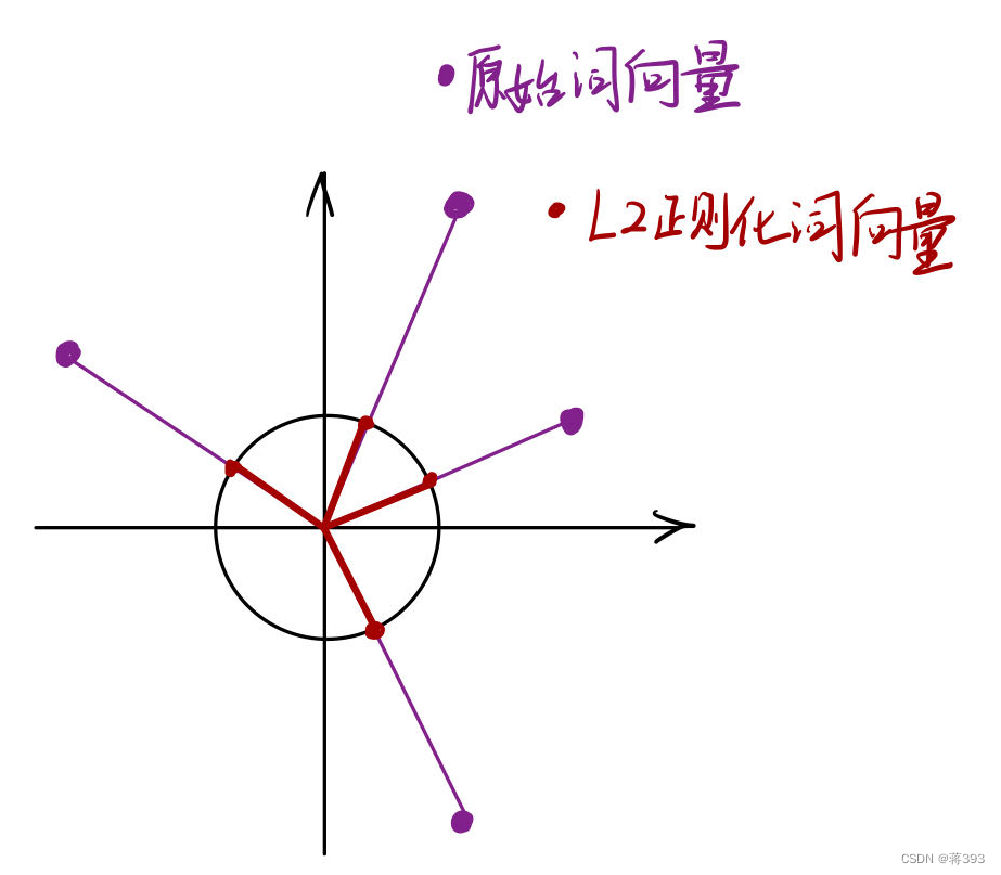
L2正则化原理如图所示,将向量转换为单位向量,其方向保持不变,但其长度被标准化为1。
L2正则化特殊情况
因此如图两个向量会使得下游任务丧失有用信息。
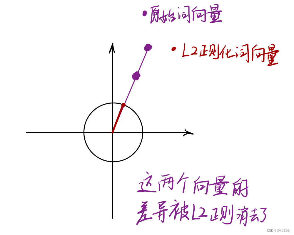
因此,在 的时候,两个向量会使得下游任务丧失有用信息。
d)对uw偏导数计算
Compute the partial derivatives of with respect to each of the 'outside' word vectors,
. There will be two cases: when
, the true 'outside' word vector, and
, for all other words. Please write your answer in terms of
,
, and
. In this subpart, you may use specific elements within these terms as well (such as
). Note that
is a vector while
are scalars. Show your work to receive full credit.
如b-i所述,
情况1: 
对正确的词向量
因为
情况2:
因为 :
e)对U的偏导数计算
Write down the partial derivative of with respect to
. Please break down your answer in terms of the column vectors
. No derivations are necessary, just an answer in the form of a matrix.
相对于 \( U \) 的偏导数可以表示为:
每个列向量 为:
对于:
对于 :
偏导数矩阵为:
任务2 机器学习与神经网络
a)adam优化器
where: is the current timestep,
is a vector containing all of the model parameters
is the model parameter at time step
, and
is the model parameter at time step
,
is the loss function,
is the gradient of the loss function with respect to the parameters on a minibatch of data,
is the learning rate.
此段回忆了最传统简单的优化器SGD(随机梯度下降算法),每进行一次迭代,都在原有基础上减去一个梯度(呼应任务1-b-iii)。adam优化器则在这个步骤上加上了两个步骤。
Adam Optimization uses a more sophisticated update rule with two additional steps.
i. momentum
First, Adam uses a trick called momentum by keeping track of \( m \), a rolling average of the gradients:
动量步骤:
改善梯度优化策略:
where is a hyperparameter between 0 and 1 (often set to 0.9).
对比SGD优化器和Adam优化器的两个递推式(下式及上式)。动量算法(不确定这个翻译是否准确)通过给之前的梯度一个权重 来计算梯度的滚动平均值。这样做可以平滑梯度,减少更新的波动。这就像是把当前梯度和之前的梯度结合起来考虑,使得更新更加稳定,避免了梯度方向的剧烈变化,更难因为随机性而陷入局部最优。
关于滚动平均值
假设我们有以下数据序列:,并且平滑系数
。通过滚动平均值计算,能够得到一系列更平滑的数据
。
ii. 自适应学习率
Adam extends the idea of momentum with the trick of adaptive learning rates by keeping track of , a rolling average of the magnitudes of the gradients:
动量步骤:
自适应步骤:
改善梯度优化策略:
where and
denote elementwise multiplication and division (so
is elementwise squaring) and
is a hyperparameter between 0 and 1 (often set to 0.99).
自适应学习率步骤通过计算梯度平方的滚动平均值,动态调整每个参数的学习率。
是当前时间步
的梯度。因此,
是梯度的平方。(
表示元素对位相乘)。对比
相关的部分,与
相关部分相似。这两部分都是使用滚动平均值,平滑优化过程。
Adam 将更新除以 ,那些具有较小梯度幅度的参数(即
较小的参数)会得到较大的更新。这防止参数更新过慢或过快,从而提高学习的收敛速度和稳定性。(这里可以想象一下
的函数图像)
通过此步骤的调整,可以防止梯度爆炸并加速收敛。
b)dropout
Dropout is a regularization technique. During training, dropout randomly sets units in the hidden layer to zero with probability
(dropping different units each minibatch), and then multiplies
by a constant
. We can write this as:
where is the size of
is a mask vector where each entry is 0 with probability
and 1 with probability
.
is chosen such that the expected value of
is
:
for all .
首先解释dropout算法。这个算法是随机将部分隐藏层的神经元关闭,随机概率是 ,这个步骤还是能够缓解神经网络的老问题:过拟合、梯度爆炸、陷入局部最优。上文中
这个式子为一个随机形成的掩码,来完成随机关闭神经元的步骤。(随机关闭导致输出结果不同的问题通过
来解决,其在后文 i 中解释)
i. 问题:What must  equal in terms of
  ?
?
Briefly justify your answer or show your math derivation using the equations given above.
题目问 等于什么,怎么证明。因为随机关闭部分隐藏层神经元,因此会导致输出和开放全部神经元的输出不同,因此需要在留存的神经元上乘以参数
,
的数值应当保证关闭部分神经元后的期望输出和原输出相同。
计算期望值
因为 以
的概率为 0,以
的概率为 1:
所以:
确保期望值等于原始值
我们希望确保 。因此,我们需要:
将等式两边同时除以 (假设
):
所以:
ii. 问题:Why should dropout be applied during training? Why should dropout NOT be applied during evaluation?
Hint: it may help to look at the dropout paper linked.
训练时使用dropout很好理解,上文也进行阐释。评估时候不用dropout 因为评估时真实评价所训练出的模型的全部能力。如果继续应用 Dropout,模型的输出会因为随机丢弃单元而不一致。
任务3
在本任务中,将实现一个基于神经网络的依存句法分析器,目标是最大化 UAS(未标注依存关系准确率)指标的表现。
一个依存句法分析器分析句子的语法结构,建立词语之间的依存关系。依存句法分析器有多种类型,包括基于转换的分析器、基于图的分析器和基于特征的分析器。你的实现将是一个基于转换的分析器,它一步一步地增量构建解析。在每一步中,它维护一个部分解析,表示如下:
- 一个当前正在处理的词语栈。
- 一个尚未处理的词语缓冲区。
- 一个由分析器预测的依存关系列表。
最初,栈中只包含 ROOT,依存关系列表为空,缓冲区包含句子的所有词语,按顺序排列。在每一步中,解析器对部分解析应用一个转换,直到其缓冲区为空且栈的大小为 1。可以应用以下转换:
- SHIFT:将缓冲区中的第一个词移出并推入栈。
- LEFT-ARC:将栈中第二个(最近添加的第二个)项目标记为第一个项目的依存项,并将第二个项目移出栈,将第一个词→第二个词的依存关系添加到依存关系列表中。
- RIGHT-ARC:将栈中第一个(最近添加的第一个)项目标记为第二个项目的依存项,并将第一个项目移出栈,将第二个词→第一个词的依存关系添加到依存关系列表中。
a)依存分析流程
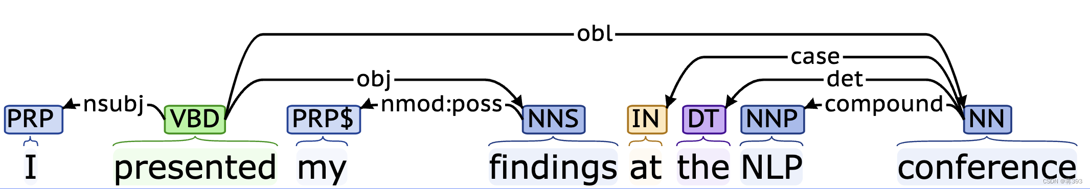
如图为一个依存关系示例。其中核心词为动词presented,依存presented的是主语I、宾语findings、地点状语conference。此问需要列出这个依存关系的生成过程。
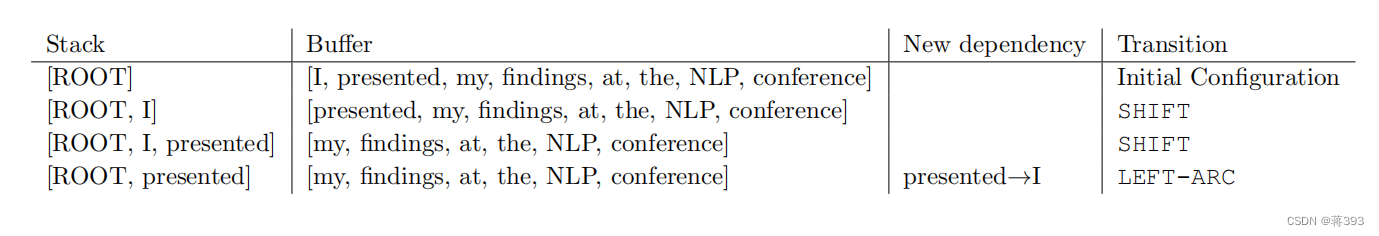
例子如图所示,后文均根据这个步骤重复即可。也就是程序需要做的初始步骤是:首先将 I 入栈,将presented入栈,用LEFT-ARC标记presented和 I 的依存关系,并且将 I 出栈。
b)迭代次数分析
每个句子中的每个单词都需要一个 SHIFT 操作将其从缓冲区移到栈中,因此有 n 次 SHIFT 操作。每个单词,还需要进行一个 LEFT-ARC 或 RIGHT-ARC 操作将其从栈中移除。因此,总共需要 2n 步来解析一个包含 n 个词的句子。
c-f)题需要完成代码
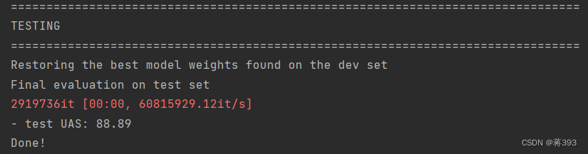
笔记记录在代码之中了,还未整理,待整理好另外发出。训练结果如下:


 2620
2620

 被折叠的 条评论
为什么被折叠?
被折叠的 条评论
为什么被折叠?
 到【灌水乐园】发言


