DiffusionFastForward(一) | Diffusion Sandbox

! git clone https://github.com/mikonvergence/DiffusionFastForward
!pip install pytorch-lightning==1.9.3 diffusers einops kornia

本文章基于Github上的DiffusionFastForward，对其中的代码进行中文介绍

import torch
import torch.nn.functional as F
import numpy as np
import matplotlib as mpl
import matplotlib.pyplot as plt
import imageio#图像处理

mpl.rcParams['figure.figsize'] = (12, 8)#修改默认图形大小

img = torch.FloatTensor(imageio.imread('./DiffusionFastForward/imgs/hills_2.png')/255)#读取一张图片，并将像素值从0-255缩小至0-1
plt.imshow(img)

定义一个自动展示图片的函数，将[0,1]转换到[-1,1]再进行输出

def input_T(input):
    # [0,1] -> [-1,+1]
    return 2*input-1
    
def output_T(input):
    # [-1,+1] -> [0,1]
    return (input+1)/2

def show(input):
    plt.imshow(output_T(input).clip(0,1))
    
img_=input_T(img)
show(img_)

如何添加和控制噪声是通过预先设定的方差时间表来实现的。

定义方差时间表：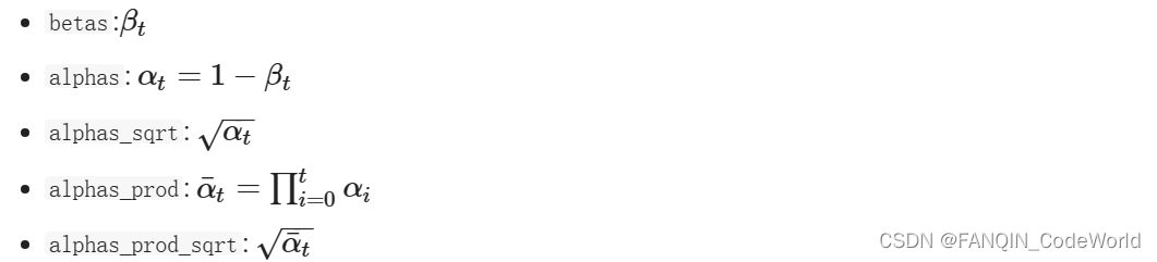

num_timesteps=1000
betas=torch.linspace(1e-4,2e-2,num_timesteps)

alphas=1-betas
alphas_sqrt=alphas.sqrt()
alphas_cumprod=torch.cumprod(alphas,0)
alphas_cumprod_sqrt=alphas_cumprod.sqrt()

利用torch.linspace()生成了一个范围为1e-4到2e-2，步数为1000的等差数列

torch.cumpord(alphas,0)计算了 alphas 按元素累积乘积，即第一个元素保持不变，第二个元素为第一个元素与第二个元素的乘积，第三个元素为前两个元素的乘积，依此类推。

前向过程：

def forward_step(t, condition_img, return_noise=False):
    """
        forward step: t-1 -> t
    """    
    assert t >= 0

    mean=alphas_sqrt[t]*condition_img    
    std=betas[t].sqrt()
      
    # sampling from N
    if not return_noise:
        return mean+std*torch.randn_like(img)
    else:
        noise=torch.randn_like(img)
        return mean+std*noise, noise
    
def forward_jump(t, condition_img, condition_idx=0, return_noise=False):
    """
        forward jump: 0 -> t
    """   
    assert t >= 0
    
    mean=alphas_cumprod_sqrt[t]*condition_img
    std=(1-alphas_cumprod[t]).sqrt()
      
    # sampling from N
    if not return_noise:
        return mean+std*torch.randn_like(img)
    else:
        noise=torch.randn_like(img)
        return mean+std*noise, noise

定义一个名为 `forward_step` 的函数，用于执行 t-1->t 的步骤。

1. `assert t >= 0`：断言语句，用于确保 t 的值大于等于 0，如果不满足则会引发 AssertionError。

2. `mean = alphas_sqrt[t] * condition_img`：计算当前时间步 t 的均值，其中 `alphas_sqrt` 是之前计算得到的系数序列，`condition_img` 是输入的条件图像。

3. `std = betas[t].sqrt()`：计算当前时间步 t 的标准差，其中 `betas` 是之前计算得到的系数序列。

4. `if not return_noise:`：判断是否需要返回噪声。如果 `return_noise` 为 False，则执行下面的代码块；否则，执行 else 语句块。

5. `return mean + std * torch.randn_like(img)`：如果不需要返回噪声，则按照标准正态分布生成一个与 `img` 相同大小的随机张量，并与均值和标准差相乘后的结果相加，最后返回这个结果。

这个函数看起来是用于在某种模型中执行前向传播的步骤，根据时间步 t、条件图像和噪声参数生成新的输出。

forward_jump 函数同理但执行 0->t 的步骤。

前向过程部分展示：

plt.figure(figsize=(12,8))
for idx in range(N):
    t_step=int(idx*(num_timesteps/N))#把一千步均匀分成了5个起点
    
    plt.subplot(N,1+M,1+(M+1)*idx)
    show(alphas_cumprod_sqrt[t_step]*img_)
    plt.title(r'$\mu_t=\sqrt{\bar{\alpha}_t}x_0$') if idx==0 else None
    plt.ylabel("t: {:.2f}".format(t_step/num_timesteps))
    plt.xticks([])
    plt.yticks([])
    
    for sample in range(M):
        x_t=forward_jump(t_step+sample,img_)
        
        plt.subplot(N,1+M,2+(1+M)*idx+sample)
        show(x_t)        
        plt.axis('off')
        
plt.tight_layout()

plit.subplot(N,1+M,1+(M+1)*idx)表示子图行数为N，列数为1+M，当前子图索引为1+(M+1)*idx。

plt.axis('off')用于隐藏坐标轴。具体地说，它会将当前图形的 x 轴和 y 轴的坐标轴线以及刻度标签都隐藏起来，使得图形只显示数据内容，而不显示坐标轴。

查看单步前向过程

plt.figure(figsize=(12,8))
for idx in range(N):
    t_step=int(idx*(num_timesteps/N))
    prev_img=forward_jump(max([0,t_step-1]),img_) # directly go to prev state
    
    plt.subplot(N,1+M,1+(M+1)*idx)
    show(alphas_sqrt[t_step]*prev_img)
    plt.title(r'$\mu_t=\sqrt{1-\beta_t}x_{t-1}$') if idx==0 else None
    plt.ylabel("t: {:.2f}".format(t_step/num_timesteps))
    plt.xticks([])
    plt.yticks([])
    
    for sample in range(M):
        plt.subplot(N,1+M,2+(1+M)*idx+sample)
        x_t=forward_step(t_step+sample,prev_img)
        show(x_t)        
        plt.axis('off')
plt.tight_layout()

反向过程：

查看加入的噪声

t_step=50

x_t,noise=forward_jump(t_step,img_,return_noise=True)

plt.subplot(1,3,1)
show(img_)
plt.title(r'$x_0$')
plt.axis('off')
plt.subplot(1,3,2)
show(x_t)
plt.title(r'$x_t$')
plt.axis('off')
plt.subplot(1,3,3)
show(noise)
plt.title(r'$\epsilon$')
plt.axis('off')

通过之前查看的噪声ε，和xt来获得x0（当然能获得平均绝对误差为0的x0）式(5)

x_0_pred=(x_t-(1-alphas_cumprod[t_step]).sqrt()*noise)/(alphas_cumprod_sqrt[t_step])

plt.subplot(1,3,1)
show(x_t)
plt.title('$x_t$ ($\ell_1$: {:.3f})'.format(F.l1_loss(x_t,img_)))
plt.axis('off')
plt.subplot(1,3,2)
show(x_0_pred)
plt.title('$x_0$ prediction ($\ell_1$: {:.3f})'.format(F.l1_loss(x_0_pred,img_)))
plt.axis('off') 
plt.subplot(1,3,3)
show(img_)
plt.title('$x_0$')
plt.axis('off')

根据和来得到的均值式(4)，并将其与真实的xt-1步的均值（前向过程中去除加噪的步骤）比较

# estimate mean
mean_pred=x_0_pred*(alphas_cumprod_sqrt[t_step-1]*betas[t_step])/(1-alphas_cumprod[t_step]) + x_t*(alphas_sqrt[t_step]*(1-alphas_cumprod[t_step-1]))/(1-alphas_cumprod[t_step])

# let's compare it to ground truth mean of the previous step (requires knowledge of x_0)
mean_gt=alphas_cumprod_sqrt[t_step-1]*img_

plt.subplot(1,3,1)
show(x_t)
plt.title('$x_t$   ($\ell_1$: {:.3f})'.format(F.l1_loss(x_t,img_)))
plt.subplot(1,3,2)
show(mean_pred)
plt.title(r'$\tilde{\mu}_{t-1}$' + '  ($\ell_1$: {:.3f})'.format(F.l1_loss(mean_pred,img_)))
plt.subplot(1,3,3)
show(mean_gt)
plt.title(r'$\mu_{t-1}$' + '  ($\ell_1$: {:.3f})'.format(F.l1_loss(mean_gt,img_)))

这个代码的思路是从xt->x0,再由xt、x0->μt-1，由μt-1加上方差即得xt-1

将上面的步骤合并就是函数reverse_step()

def reverse_step(epsilon, x_t, t_step, return_noise=False):
    
    # estimate x_0 based on epsilon
    x_0_pred=(x_t-(1-alphas_cumprod[t_step]).sqrt()*epsilon)/(alphas_cumprod_sqrt[t_step])
    if t_step==0:
        sample=x_0_pred
        noise=torch.zeros_like(x_0_pred)
    else:
        # estimate mean
        mean_pred=x_0_pred*(alphas_cumprod_sqrt[t_step-1]*betas[t_step])/(1-alphas_cumprod[t_step]) + x_t*(alphas_sqrt[t_step]*(1-alphas_cumprod[t_step-1]))/(1-alphas_cumprod[t_step])

        # compute variance
        beta_pred=betas[t_step].sqrt() if t_step != 0 else 0

        sample=mean_pred+beta_pred*torch.randn_like(x_t)
        # this noise is only computed for simulation purposes (since x_0_pred is not known normally)
        #使用式(4)得到噪音
        noise=(sample-x_0_pred*alphas_cumprod_sqrt[t_step-1])/(1-alphas_cumprod[t_step-1]).sqrt()
    if return_noise:
        return sample, noise
    else:
        return sample

x_t,noise=forward_jump(1000-1,img_,return_noise=True)

state_imgs=[x_t.numpy()]
for t_step in reversed(range(1000)):
    x_t,noise=reverse_step(noise,x_t,t_step,return_noise=True)
    
    if t_step % 200 == 0:
        state_imgs.append(x_t.numpy())

可以通过以上代码来验证reverse函数，但需要注意的是，此时仍然未完成diffusion，甚至可以说仅仅只是冰山一角。其原因是，上述代码已知了图片img_然后利用img_得到x_t和noise，事实上由这两个可以直接得到img_，而不需要经过一个reverse过程，因此这里的代码只是形象的展示了一下diffusion的过程，未涉及到模型的训练过程。