


5.0程序运行前的库
import pandas as pd
import numpy as np
import statsmodels.api as sm
import matplotlib.pyplot as plt
from statsmodels.stats.outliers_influence import variance_inflation_factor
5.1引言
定性变量可以用实型变量或虚拟变量来表示,对于定性变量,其一般取值为0或1,表明观测属于两个可能类别中的一个;示性变量也可以区分3个或3个以上的类别
5.2薪水调查数据
(一)目的:明确并量化那些决定薪水差异的变量;也可用来检验公司的薪水管理制度是否得到遵行
(二)响应变量为薪水S;预测变量:工作年数X,教育E[高中1,硕士2,更高3],管理M[人在管理职位1;其他职位0]
两个示性变量表示三种教育水平,这两个变量使得我们可以衡量受教育水平对薪水差异的影响
data1=pd.read_csv('F:\linear  regression\chapter 5\Table 5.1.csv')
data1.columns=['S','X','E','M']#X工作年数,E教育,M为是否为在职管理者
E=data1['E']
X=data1['X']
# 我们需要对表格中的数据进行定性的表示
这样做的目的:用来区分两个管理类别的示性变量只需要一个,示性变量取值为0的类别为基础类别,因为示性变量的回归系数是相对于对照组的增量
#哑变量 示性变量
#首先我们将定性变量E转换为虚拟变量
dummies=pd.get_dummies(data1['E'],'E')
#将E列展开,对E中插入我们想要的列表的数据
#读取第1列的值
#读取第2列的值
data1.insert(2,'E_1',dummies.iloc[:,0])
data1.insert(3,'E_2',dummies.iloc[:,1])
data1.insert(1,'constant',1)
#去掉哑变量
data1=data1.drop('E',axis=1)#删除其中的E教育所在行列,用0,1来表示
data1
Table 5.3 Regression Analysis of Salary Survey Data
ols_1=(sm.OLS(data1['S'],data1[data1.columns[1:6]].astype(float))).fit()
print(ols_1.summary())
OLS Regression Results
==============================================================================
Dep. Variable: S R-squared: 0.957
Model: OLS Adj. R-squared: 0.953
Method: Least Squares F-statistic: 226.8
Date: Wed, 13 Dec 2023 Prob (F-statistic): 2.23e-27
Time: 21:59:45 Log-Likelihood: -381.63
No. Observations: 46 AIC: 773.3
Df Residuals: 41 BIC: 782.4
Df Model: 4
Covariance Type: nonrobust
==============================================================================
coef std err t P>|t| [0.025 0.975]
------------------------------------------------------------------------------
constant 1.103e+04 383.217 28.787 0.000 1.03e+04 1.18e+04
X 546.1840 30.519 17.896 0.000 484.549 607.819
E_1 -2996.2103 411.753 -7.277 0.000 -3827.762 -2164.659
E_2 147.8249 387.659 0.381 0.705 -635.069 930.719
M 6883.5310 313.919 21.928 0.000 6249.559 7517.503
==============================================================================
Omnibus: 2.293 Durbin-Watson: 2.237
Prob(Omnibus): 0.318 Jarque-Bera (JB): 1.362
Skew: -0.077 Prob(JB): 0.506
Kurtosis: 2.171 Cond. No. 35.4
==============================================================================
from scipy.stats import t,f
t(41).isf(0.025)
2.019540963982894
5.3 交互作用变量
模型设定问题
Figure 5.1 对工作年数的标准化残差图
首先这幅图存在三个或多个的残差水平。
outliers=ols_1.get_influence()
res1=outliers.resid_studentized_internal
plt.scatter(data1['X'],res1)
plt.xlabel('X')
plt.ylabel('Residuals')
plt.title('Figure 5.1')
plt.show()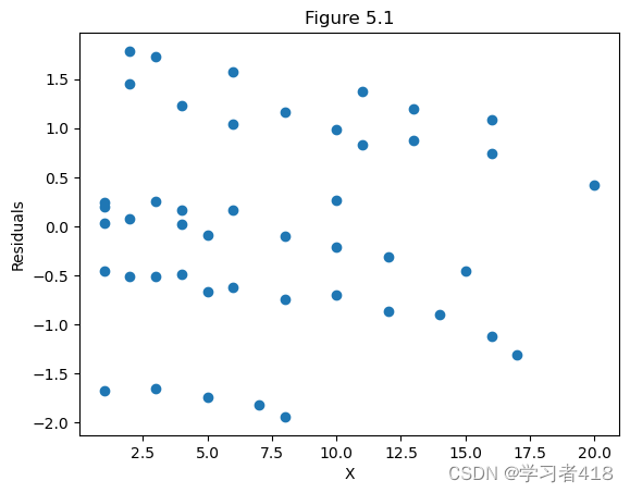
Figure 5.2 对E-M组合类别变量的标准化残差图
分为6种;从表中不难发现:残差或者几乎全为正或者几乎全为负,这表明给出的模型并未充分解释薪水和工作年数,教育,以及管理变量之间的关系【总的概括而言:数据中一些隐含的数据结构并未被挖掘出来】
em=-1+2*E+data1['M']
plt.scatter(em,res1)
plt.xlabel('Catagory')
plt.ylabel('Residuals')
plt.title('Figure 5.2')
plt.show()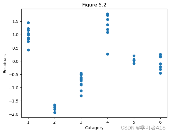
Table 5.4 扩展模型
教育和管理两者不可加,但却承认两个变量有交互效应的模型
data1['E1M']=data1['E_1']*data1['M']
data1['E2M']=data1['E_2']*data1['M']
data1
(一)首先,我们对扩展后的模型有一个初步的了解,先做回归分析
ols_2=(sm.OLS(data1['S'],data1[data1.columns[1:]].astype(float))).fit()
print(ols_2.summary())
OLS Regression Results
==============================================================================
Dep. Variable: S R-squared: 0.999
Model: OLS Adj. R-squared: 0.999
Method: Least Squares F-statistic: 5517.
Date: Wed, 13 Dec 2023 Prob (F-statistic): 1.67e-55
Time: 21:59:53 Log-Likelihood: -298.74
No. Observations: 46 AIC: 611.5
Df Residuals: 39 BIC: 624.3
Df Model: 6
Covariance Type: nonrobust
==============================================================================
coef std err t P>|t| [0.025 0.975]
------------------------------------------------------------------------------
constant 1.12e+04 79.065 141.698 0.000 1.1e+04 1.14e+04
X 496.9870 5.566 89.283 0.000 485.728 508.246
E_1 -1730.7483 105.334 -16.431 0.000 -1943.806 -1517.690
E_2 -349.0777 97.568 -3.578 0.001 -546.427 -151.728
M 7047.4120 102.589 68.695 0.000 6839.906 7254.918
E1M -3066.0351 149.330 -20.532 0.000 -3368.084 -2763.986
E2M 1836.4879 131.167 14.001 0.000 1571.177 2101.799
==============================================================================
Omnibus: 74.761 Durbin-Watson: 2.244
Prob(Omnibus): 0.000 Jarque-Bera (JB): 1037.873
Skew: -4.103 Prob(JB): 4.25e-226
Kurtosis: 24.776 Cond. No. 83.4
==============================================================================
Figur 5.3 扩展模型对工作年数的标准化残差图
此模型过高预测了这一点上的薪水,检查原数据集这个观测,发现这个人比其他特征相似的人年薪低几百元,为了确保这一观测不过度影响回归估计,将它去掉重新做回归
n=len(X)
index=np.arange(1,46)
outliers=ols_2.get_influence()
res2=outliers.resid_studentized_internal
#找出outliers
col=[]
for i in range(0,n):
    if abs(res2[i])>2:
        col.append('r')
        plt.annotate(index[i],xy=(X[i],res2[i]))#散点图注释
    else:
        col.append('b')
plt.scatter(X,res2,c=col)
plt.xlabel('X')
plt.ylabel('Resdual')
plt.title('index plot of resduals:expanded model')
plt.show()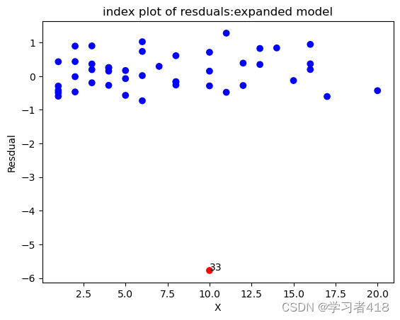
outlier 为第33个观测值,需要删除
data1_1=data1.drop(32,axis=0)#第1列的第33个观测值
ols_3=(sm.OLS(data1_1['S'],data1_1[data1_1.columns[1:]].astype(float))).fit()
print(ols_3.summary())
OLS Regression Results
==============================================================================
Dep. Variable: S R-squared: 1.000
Model: OLS Adj. R-squared: 1.000
Method: Least Squares F-statistic: 3.543e+04
Date: Wed, 13 Dec 2023 Prob (F-statistic): 1.30e-69
Time: 21:59:56 Log-Likelihood: -249.34
No. Observations: 45 AIC: 512.7
Df Residuals: 38 BIC: 525.3
Df Model: 6
Covariance Type: nonrobust
==============================================================================
coef std err t P>|t| [0.025 0.975]
------------------------------------------------------------------------------
constant 1.12e+04 30.533 366.802 0.000 1.11e+04 1.13e+04
X 498.4178 2.152 231.640 0.000 494.062 502.774
E_1 -1741.3359 40.683 -42.803 0.000 -1823.693 -1658.979
E_2 -357.0423 37.681 -9.475 0.000 -433.324 -280.761
M 7040.5801 39.619 177.707 0.000 6960.376 7120.785
E1M -3051.7633 57.674 -52.914 0.000 -3168.519 -2935.008
E2M 1997.5306 51.785 38.574 0.000 1892.697 2102.364
==============================================================================
Omnibus: 1.462 Durbin-Watson: 2.438
Prob(Omnibus): 0.482 Jarque-Bera (JB): 1.171
Skew: 0.177 Prob(JB): 0.557
Kurtosis: 2.293 Cond. No. 82.5
==============================================================================
Figure 5.4
删除第33个观测值的扩展模型中对X的标准化残差 新的残差图与原可加模型类似的残差图相比更令人满意
outliers=ols_3.get_influence()
res3=outliers.resid_studentized_internal
plt.scatter(data1_1['X'],res3)
plt.xlabel('X')
plt.ylabel('Residuals')
plt.title('Figure 5.4')
plt.show()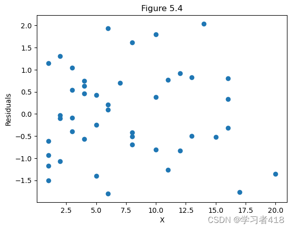
对EM组合变量的标准化残差(扩展,删33)
每个组合类的残差关于0的分布对称
E=E.drop(32)
EM=-1+2*E+data1_1['M']
plt.scatter(EM,res3)
plt.xlabel('Category',size=13)
plt.ylabel('Residuals',size=13)
plt.title('Figure 5.5',size=15)
plt.show()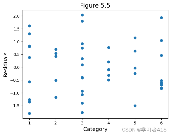
求取对应的t值
from scipy.stats import t,f
t(38).isf(0.025)
2.0243941645751367
beta=ols_3.params
x0=np.vstack([[1,1,1,1,1,1],[0,0,0,0,0,0],[1,1,0,0,0,0],[0,0,1,1,0,0],[0,1,0,1,0,1],[0,1,0,0,0,0],[0,0,0,1,0,0]]).T
yuce=x0.dot(beta)

#计算标准误
X=data1_1[['constant','X','E_1','E_2','M','E1M','E2M']].values
fit=ols_3.fittedvalues
sigma=((np.sum((data1_1['S']-fit)**2))/38)**0.5
s_e=[]
for i in range(6):
    x01=x0[i,:].reshape(7,1)
    se=x01.T.dot(np.linalg.inv(X.T.dot(X))).dot(x01)
    se=((se+1)**0.5)*sigma
    s_e.insert(i,float(se))

#计算预测值的预测区间
upper=[]
lower=[]
for i in range(6):
    upper.insert(i,yuce[i]+t.isf(0.025,38)*s_e[i])
    lower.insert(i,yuce[i]-t.isf(0.025,38)*s_e[i])

table=pd.DataFrame()
table['category']=[1,2,3,4,5,6]
table['estimate']=yuce
table['se']=s_e
table['CI_lower']=lower
table['CI_upper']=upper
table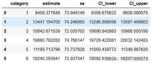
5.4 回归方程系统:两个组的比较
5.4.0数据导入以及需要用到的库
import pandas as pd
import numpy as np
import statsmodels.api as sm
import matplotlib.pyplot as plt
from statsmodels.stats.outliers_influence import variance_inflation_factor
data2=pd.read_csv('F:\linear  regression\chapter 5\Table 5.7.csv')
data2.columns=['TEST','RACE','JPERF']
RACE=data2['RACE']
JPERF=data2['JPERF']
data2.insert(1,'constant',1)
ols_4=(sm.OLS(data2['JPERF'],data2[['constant','TEST']].astype(float))).fit()
print(ols_4.summary())OLS Regression Results
==============================================================================
Dep. Variable: JPERF R-squared: 0.517
Model: OLS Adj. R-squared: 0.490
Method: Least Squares F-statistic: 19.25
Date: Wed, 13 Dec 2023 Prob (F-statistic): 0.000356
Time: 22:09:05 Log-Likelihood: -36.614
No. Observations: 20 AIC: 77.23
Df Residuals: 18 BIC: 79.22
Df Model: 1
Covariance Type: nonrobust
==============================================================================
coef std err t P>|t| [0.025 0.975]
------------------------------------------------------------------------------
constant 1.0350 0.868 1.192 0.249 -0.789 2.859
TEST 2.3605 0.538 4.387 0.000 1.230 3.491
==============================================================================
Omnibus: 0.324 Durbin-Watson: 2.896
Prob(Omnibus): 0.850 Jarque-Bera (JB): 0.483
Skew: -0.186 Prob(JB): 0.785
Kurtosis: 2.336 Cond. No. 5.26
==============================================================================
from prettytable import PrettyTable#创建表格
label1=['Source','Sum of Squares','d.f.','Mean Square']
table=PrettyTable(label1)
table.add_row(['Regression',ols_4.df_model*ols_4.mse_model,ols_4.df_model,ols_4.mse_model])
table.add_row(['Residuals',ols_4.ssr,ols_4.df_resid,ols_4.mse_resid])
table.add_column('F',[ols_4.fvalue,'--'])
print(table)
+------------+--------------------+------+--------------------+------------------+
|   Source   |   Sum of Squares   | d.f. |    Mean Square     |        F         |
+------------+--------------------+------+--------------------+------------------+
| Regression |  48.7229581716978  | 1.0  |  48.7229581716978  | 19.2461274204537 |
| Residuals  | 45.568296828302195 | 18.0 | 2.5315720460167888 |        --        |
+------------+--------------------+------+--------------------+------------------+
data2['RACE*TEST']=data2['RACE']*data2['TEST']
ols_5=(sm.OLS(data2['JPERF'],data2[['constant','TEST','RACE','RACE*TEST']].astype(float))).fit()
print(ols_5.summary())
OLS Regression Results
==============================================================================
Dep. Variable: JPERF R-squared: 0.664
Model: OLS Adj. R-squared: 0.601
Method: Least Squares F-statistic: 10.55
Date: Wed, 13 Dec 2023 Prob (F-statistic): 0.000451
Time: 22:09:06 Log-Likelihood: -32.971
No. Observations: 20 AIC: 73.94
Df Residuals: 16 BIC: 77.92
Df Model: 3
Covariance Type: nonrobust
==============================================================================
coef std err t P>|t| [0.025 0.975]
------------------------------------------------------------------------------
constant 2.0103 1.050 1.914 0.074 -0.216 4.236
TEST 1.3134 0.670 1.959 0.068 -0.108 2.735
RACE -1.9132 1.540 -1.242 0.232 -5.179 1.352
RACE*TEST 1.9975 0.954 2.093 0.053 -0.026 4.021
==============================================================================
Omnibus: 3.377 Durbin-Watson: 3.015
Prob(Omnibus): 0.185 Jarque-Bera (JB): 1.330
Skew: 0.120 Prob(JB): 0.514
Kurtosis: 1.760 Cond. No. 13.8
==============================================================================
label2=['Source','Sum of Squares','d.f.','Mean Square']
table=PrettyTable(label2)
table.add_row(['Regression',ols_5.df_model*ols_5.mse_model,ols_5.df_model,ols_5.mse_model])
table.add_row(['Residuals',ols_5.ssr,ols_5.df_resid,ols_5.mse_resid])
table.add_column('F',[ols_5.fvalue,'--'])
print(table)
+------------+-------------------+------+-------------------+-------------------+ | Source | Sum of Squares | d.f. | Mean Square | F | +------------+-------------------+------+-------------------+-------------------+ | Regression | 62.63578183766151 | 3.0 | 20.87859394588717 | 10.55291454406796 | | Residuals | 31.65547316233848 | 16.0 | 1.978467072646155 | -- | +------------+-------------------+------+-------------------+-------------------+
Figure 5.7 Model 1 对测试得分的标准化残差图
outliers=ols_4.get_influence()
res4=outliers.resid_studentized_internal
plt.scatter(data2['TEST'],res4)
plt.xlabel('TEST',size=13)
plt.ylabel('Residuals',size=13)
plt.title('Figure 5.7',size=15)
plt.show()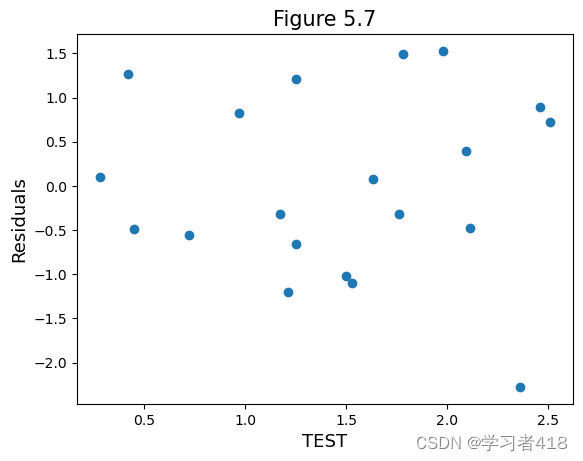
Figure 5.8 Model 3 对测试得分的标准化残差图
outliers=ols_5.get_influence()
res5=outliers.resid_studentized_internal
plt.scatter(data2['TEST'],res5)
plt.xlabel('TEST',size=13)
plt.ylabel('Residuals',size=13)
plt.title('Figure 5.8',size=15)
plt.show()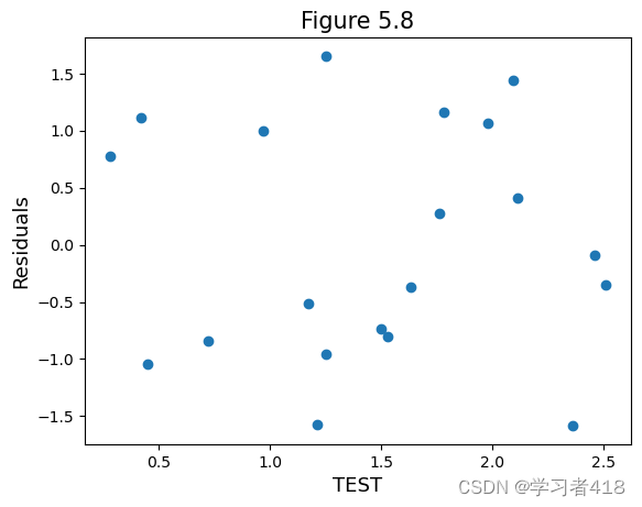
Figure 5.9 对Model 1 种族的标准化残差图
plt.scatter(data2['RACE'],res4)
plt.xlabel('RACE')
plt.ylabel('Residuals')
plt.title('Figure 5.9')
plt.show()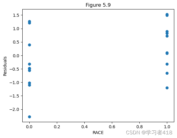
from scipy.stats import t,f
f.isf(0.05,2,16)
3.63372346759163
SSE_4=sum(res4**2)
SSE_5=sum(res5**2)
print(SSE_4)
print(SSE_5)
20.02709825217295 19.806440174731453
results_1=(sm.OLS(data2.iloc[0:10,3],data2.iloc[0:10,0:2])).fit()
print(results_1.summary())
results_2=(sm.OLS(data2.iloc[10:20,3],data2.iloc[10:20,0:2])).fit()
print(results_2.summary())
OLS Regression Results
==============================================================================
Dep. Variable: JPERF R-squared: 0.779
Model: OLS Adj. R-squared: 0.751
Method: Least Squares F-statistic: 28.14
Date: Wed, 13 Dec 2023 Prob (F-statistic): 0.000724
Time: 22:20:37 Log-Likelihood: -15.637
No. Observations: 10 AIC: 35.27
Df Residuals: 8 BIC: 35.88
Df Model: 1
Covariance Type: nonrobust
==============================================================================
coef std err t P>|t| [0.025 0.975]
------------------------------------------------------------------------------
TEST 3.3109 0.624 5.305 0.001 1.872 4.750
constant 0.0971 1.035 0.094 0.928 -2.290 2.484
==============================================================================
Omnibus: 0.635 Durbin-Watson: 2.411
Prob(Omnibus): 0.728 Jarque-Bera (JB): 0.554
Skew: -0.161 Prob(JB): 0.758
Kurtosis: 1.893 Cond. No. 5.55
==============================================================================
Notes:
[1] Standard Errors assume that the covariance matrix of the errors is correctly specified.
OLS Regression Results
==============================================================================
Dep. Variable: JPERF R-squared: 0.293
Model: OLS Adj. R-squared: 0.205
Method: Least Squares F-statistic: 3.320
Date: Wed, 13 Dec 2023 Prob (F-statistic): 0.106
Time: 22:20:37 Log-Likelihood: -17.211
No. Observations: 10 AIC: 38.42
Df Residuals: 8 BIC: 39.03
Df Model: 1
Covariance Type: nonrobust
==============================================================================
coef std err t P>|t| [0.025 0.975]
------------------------------------------------------------------------------
TEST 1.3134 0.721 1.822 0.106 -0.349 2.976
constant 2.0103 1.129 1.780 0.113 -0.593 4.614
==============================================================================
Omnibus: 2.077 Durbin-Watson: 2.880
Prob(Omnibus): 0.354 Jarque-Bera (JB): 0.932
Skew: 0.294 Prob(JB): 0.627
Kurtosis: 1.624 Cond. No. 5.01
==============================================================================
Figure 5.10
#图5.10
outliers=results_1.get_influence()
res1=outliers.resid_studentized_internal
plt.scatter(data2.loc[data2['RACE']==1,'TEST'],res1)
plt.xlabel('TEST',size=13)
plt.ylabel('Residuals',size=13)
plt.title('Figure 5.10',size=15)
plt.show() 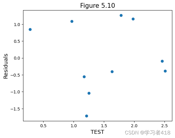
Figure 5.11
#图5.11
outliers=results_2.get_influence()
res2=outliers.resid_studentized_internal
plt.scatter(data2.loc[data2['RACE']==0,'TEST'],res2)
plt.xlabel('TEST',size=13)
plt.ylabel('Residuals',size=13)
plt.title('Figure 5.11',size=15)
plt.show()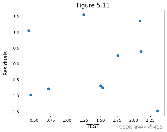
ols_6=(sm.OLS(data2['JPERF'],data2[['constant','TEST','RACE']].astype(float))).fit()
print(ols_6.summary())
OLS Regression Results
==============================================================================
Dep. Variable: JPERF R-squared: 0.572
Model: OLS Adj. R-squared: 0.522
Method: Least Squares F-statistic: 11.38
Date: Sun, 17 Dec 2023 Prob (F-statistic): 0.000731
Time: 19:18:40 Log-Likelihood: -35.390
No. Observations: 20 AIC: 76.78
Df Residuals: 17 BIC: 79.77
Df Model: 2
Covariance Type: nonrobust
==============================================================================
coef std err t P>|t| [0.025 0.975]
------------------------------------------------------------------------------
constant 0.6120 0.887 0.690 0.500 -1.260 2.483
TEST 2.2988 0.522 4.400 0.000 1.197 3.401
RACE 1.0276 0.691 1.487 0.155 -0.430 2.485
==============================================================================
Omnibus: 0.251 Durbin-Watson: 3.028
Prob(Omnibus): 0.882 Jarque-Bera (JB): 0.437
Skew: -0.059 Prob(JB): 0.804
Kurtosis: 2.286 Cond. No. 5.72
==============================================================================
Notes:
[1] Standard Errors assume that the covariance matrix of the errors is correctly specified.
label3=['Source','Sum of Squares','d.f.','Mean Square']
table=PrettyTable(label3)
table.add_row(['Regression',ols_6.df_model*ols_6.mse_model,ols_6.df_model,ols_6.mse_model])
table.add_row(['Residuals',ols_6.ssr,ols_6.df_resid,ols_6.mse_resid])
table.add_column('F',[ols_6.fvalue,'--'])
print(table)
+------------+--------------------+------+-------------------+--------------------+ | Source | Sum of Squares | d.f. | Mean Square | F | +------------+--------------------+------+-------------------+--------------------+ | Regression | 53.96970908443848 | 2.0 | 26.98485454221924 | 11.377106626278483 | | Residuals | 40.321545915561515 | 17.0 | 2.371855642091854 | -- | +------------+--------------------+------+-------------------+--------------------+
from scipy.stats import t,f
f.isf(0.05,2,16)
3.63372346759163


 2270
2270


 被折叠的 条评论
为什么被折叠?
被折叠的 条评论
为什么被折叠?
 到【灌水乐园】发言


