


💥💥💞💞欢迎来到本博客❤️❤️💥💥
🏆博主优势:🌞🌞🌞博客内容尽量做到思维缜密,逻辑清晰,为了方便读者。
⛳️座右铭:行百里者,半于九十。
📋📋📋本文目录如下:🎁🎁🎁
目录

💥1 概述
-
计算浸没式圆柱形三系波浪能转换器的发电量和平准化能量成本涉及多个因素,包括波浪资源、装置设计、转换效率等。以下是一些常见的方法和指标,可用于计算和评估浸没式圆柱形三系波浪能转换器的发电量和平准化能量成本:
-
发电量计算:
-
波浪资源评估:通过测量或模拟波浪数据,确定波浪的频率、振幅和能量密度等参数。
-
转换效率评估:根据装置设计和性能参数,估计转换器从波浪能量中提取的能量比例。
-
发电量计算:将波浪资源和转换效率结合起来,计算转换器的年发电量。这可以通过将波浪能量密度与转换效率相乘,并考虑装置的运行时间和可利用性来实现。
-
-
平准化能量成本计算:
-
投资成本评估:考虑转换器的设计、制造和安装成本,以及与之相关的基础设施和电网连接成本。
-
运维成本评估:考虑转换器的维护、修理和监控成本,以及与之相关的人力和资源成本。
-
折旧和财务成本评估:考虑转换器的寿命和折旧,以及与之相关的财务成本,如利息和税收。
-
平准化能量成本计算:将投资成本、运维成本和财务成本结合起来,除以转换器的年发电量,计算单位能量的平准化成本。
-
需要注意的是,具体的计算方法和参数取决于具体的转换器设计和运行条件。因此,建议参考相关的研究论文、技术报告或专业文献,以获取更详细和准确的计算方法和数据。此外,与该领域的专业人士进行讨论和咨询也是获取准确信息的好途径。
-
📚2 运行结果
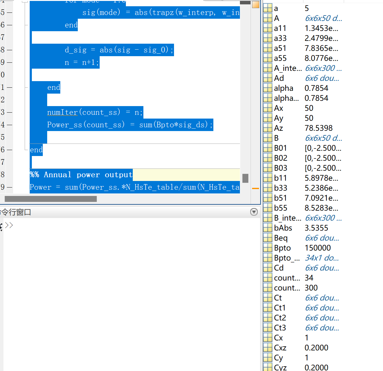
部分代码:
%% Code is written by N. Y. Sergiienko
% University of Adelaide
%% 20/11/2019 Shape optimisation
% Shape: cylinder
% Number of buoys: 1 buoy
% Fitness function: power
% Sea site: Albany
% Hydrodynamics: analytical based on Linton (1991)
% Model: spectral domain
clear;
clc;
close all;
opts = optimset('Diagnostics','off', 'Display','off');
load Albany_table
% Number of sea states
N_ss = length(Hs_table);
%% Cylinder parameters to be optimised
a = 5; % Acceptable range = 1 - 20 m
H = 5; % Acceptable range = 1 - 30 m
alpha = deg2rad(45); % Acceptable range = 10-80 deg = 0.1745 - 1.3963 rad
alphaAP = deg2rad(45); % Acceptable range = 10-80 deg = 0.1745 - 1.3963 rad
Kpto_table = 2e5*ones(N_ss, 1); % Acceptable range = 1e3 - 1e8
Bpto_table = 1.5e5*ones(N_ss, 1); % Acceptable range = 1e3 - 1e8
%%
h = 50; % water depth
ds = 2 + H/2; % submergence depth (from water level to the buoy centre)
rho = 1025; % water density
g = 9.81; % gravitational acceleration
V = pi*a^2*H; % volume
m = 0.5*V*rho; % mass
I3 = eye(3);
% Buoyancy force
Fb = (rho*V - m)*g;
Fbuoy = [0 0 Fb 0 0]';
% Mass matrix
Iz = m*a^2/2;
Ix = 1/12*m*(3*a^2+H^2);
Iy = Ix;
M = diag([m m m Ix Iy Iz]);
% Drag coefficients
Cx = 1;
Cy = 1;
Cz = -0.12*(H/a) + 1.2; % Took data from AWTEC (2016) and did a linear fit - matches well with other literature
Cxz = 0.2;
Cyz = 0.2;
Cd = diag([Cx Cy Cz Cxz Cyz 0]);
Ax = H*2*a;
Ay = Ax;
Az = pi*a^2;
D = 2*a;
Ad = diag([Ax Ay Az D^4*D D^4*D D^4*D]);
%% Hydrodynamic parameters
numFreqs = 50;
numApprox = 50;
w_min = 0.1;
w_max = 2.5;
w_array = linspace(w_min, w_max, numFreqs);
A = zeros(6,6,numFreqs);
B = zeros(6,6,numFreqs);
fexc = zeros(6,numFreqs);
for count_w = 1:length(w_array)
w = w_array(count_w);
% Hydrodynamic parameters of a submerged sphere in finite depth
k = fsolve(@(x)w^2-g*x*tanh(x*h), w^2/g*sqrt(coth(w^2/g*h)), opts);
% Hydrodynamic parameters of a submerged cylinder in finite depth
[a11, a33, a55, a51, b11, b33, b55, b51, fx, fz, My] = submergedCylinder(a, H, h, ds, k, rho, w, numApprox);
% Excitation force
fexc(:,count_w) = [fx; 0; fz; 0; My; 0];
% Added mass matrix
A(:,:,count_w) = ...
[a11 0 0 0 a51 0;
0 a11 0 a51 0 0;
0 0 a33 0 0 0;
0 a51 0 a55 0 0;
a51 0 0 0 a55 0;
0 0 0 0 0 0];
% Damping matrix
B(:,:,count_w) = ...
[b11 0 0 0 b51 0;
0 b11 0 b51 0 0;
0 0 b33 0 0 0;
0 b51 0 b55 0 0;
b51 0 0 0 b55 0;
0 0 0 0 0 0];
end
%% Interpolate data for 300 points
numFreqs_interp = 300;
A_interp = zeros(6,6,numFreqs_interp);
B_interp = zeros(6,6,numFreqs_interp);
fexc_interp = zeros(6,numFreqs_interp);
w_interp = linspace(w_min, w_max, numFreqs_interp)';
for mode_i = 1:6
for mode_j = 1:6
A_interp(mode_i, mode_j, :) = interp1(w_array, squeeze(A(mode_i, mode_j,:)), w_interp);
B_interp(mode_i, mode_j, :) = interp1(w_array, squeeze(B(mode_i, mode_j,:)), w_interp);
end
fexc_interp(mode_i, :) = interp1(w_array, fexc(mode_i, :), w_interp);
end
%% WEC model
% Linearised model of the three-tether WEC (from Scruggs)
if tan(alphaAP) > a/(H/2)
bAbs = a/sin(alphaAP);
else
bAbs = H/2/cos(alphaAP);
end
L0 = (h - ds - bAbs*cos(alphaAP))/cos(alpha);
% Unit vectors with alpha
es01 = [-sin(alpha); 0; cos(alpha)];
es02 = [sin(alpha)/2; sqrt(3)/2*sin(alpha); cos(alpha)];
es03 = [sin(alpha)/2; -sqrt(3)/2*sin(alpha); cos(alpha)];
% Unit vectors with alphaAP
es01AP = [-sin(alphaAP); 0; cos(alphaAP)];
es02AP = [sin(alphaAP)/2; sqrt(3)/2*sin(alphaAP); cos(alphaAP)];
es03AP = [sin(alphaAP)/2; -sqrt(3)/2*sin(alphaAP); cos(alphaAP)];
% Vectors on the sea floor from the centre to the attachment points
d1 = - (L0*es01 + bAbs*es01AP); d1(3) = 0;
d2 = - (L0*es02 + bAbs*es02AP); d2(3) = 0;
d3 = - (L0*es03 + bAbs*es03AP); d3(3) = 0;
% Eq.(1)
ES01 = crossV2M(es01);
ES02 = crossV2M(es02);
ES03 = crossV2M(es03);
ES01AP = crossV2M(es01AP);
ES02AP = crossV2M(es02AP);
ES03AP = crossV2M(es03AP);
% Attachment point of tethers
n01 = -bAbs*es01AP;
n02 = -bAbs*es02AP;
n03 = -bAbs*es03AP;
B01 = bAbs*(-ES01AP);
B02 = bAbs*(-ES02AP);
B03 = bAbs*(-ES03AP);
s0n = L0;
S01 = ES01*s0n;
S02 = ES02*s0n;
S03 = ES03*s0n;
% Initial tention in a leg - function of an inclination angle
t0(1,1) = Fb/(3*cos(alpha));
t0(2,1) = Fb/(3*cos(alpha));
t0(3,1) = t0(2,1);
gam0 = t0/s0n;
% Kt and Ct from Scruggs (2013)
% Eq.11
Gt1 = (-[I3; B01']*es01);
Gt2 = (-[I3; B02']*es02);
Gt3 = (-[I3; B03']*es03);
%% Loop over all sea states
Power_ss = zeros(N_ss, 1);
for count_ss = 1:N_ss
Hs = Hs_table(count_ss);
Tp = Te_table(count_ss)/0.858;
% Wave spectrum for this sea state
Spec = spectrum_PM_n(Hs, Tp, w_interp);
Sw = Spec.data;
%% PTO matrices for this sea state
Kpto = Kpto_table(count_ss);
Bpto = Bpto_table(count_ss);
% Eq.13
Ct1 = Bpto*(Gt1*Gt1');
Ct2 = Bpto*(Gt2*Gt2');
Ct3 = Bpto*(Gt3*Gt3');
% Eq.14
Kt1 = ((Kpto-gam0(1))*(Gt1*Gt1') + gam0(1)*[I3; B01']*[I3 B01] + [zeros(3) zeros(3); zeros(3) gam0(1)*S01*B01]);
Kt2 = ((Kpto-gam0(2))*(Gt2*Gt2') + gam0(2)*[I3; B02']*[I3 B02] + [zeros(3) zeros(3); zeros(3) gam0(2)*S02*B02]);
Kt3 = ((Kpto-gam0(3))*(Gt3*Gt3') + gam0(3)*[I3; B03']*[I3 B03] + [zeros(3) zeros(3); zeros(3) gam0(3)*S03*B03]);
Ct = Ct1 + Ct2 + Ct3;
Kt = Kt1 + Kt2 + Kt3;
%% Spectral domain model
Beq = zeros(6);
n = 0;
Sq = zeros(6, 6, numFreqs_interp);
Sds = zeros(3, numFreqs_interp);
ddelta_s = zeros(3, numFreqs_interp);
% sig_0 = zeros(1,6);
sig = zeros(1,6);
d_sig = 1e6*ones(1,3);
sig_ds = zeros(1,3);
% for count_w = 1:length(w_interp)
% w = w_interp(count_w);
% Sf = Sw(count_w)*abs(fexc_interp(:, count_w)).^2;
% Hx = (-w^2*(M + A_interp(:,:,count_w)) + 1i*w*(B_interp(:,:,count_w) + Ct + Beq) + Kt)^(-1);
% Sq_SL(:,:,count_w) = Hx*diag(Sf)*Hx';
% end
%
%
% for mode = 1:6
% sig(mode) = abs(trapz(w_interp, w_interp.^2.*squeeze(Sq_SL(mode,mode,:))));
% end
while any(~(d_sig <= 0.01)) && n < 100
sig_0 = sig;
Beq = 1/2*rho*Cd*Ad*sqrt(8/pi)*diag(sig);
for count_w = 1:length(w_interp)
w = w_interp(count_w);
Sf = Sw(count_w)*abs(fexc_interp(:, count_w)).^2;
Hx_w = pinv(-w^2*(M + A_interp(:,:,count_w)) + 1i*w*(B_interp(:,:,count_w) + Ct + Beq) + Kt);
RAO = Hx_w*fexc_interp(:, count_w);
Sq(:,:,count_w) = Hx_w*diag(Sf)*Hx_w';
ddelta_s(1, count_w) = es01'*(1i*w*RAO(1:3) + B01*1i*w*RAO(4:6));
ddelta_s(2, count_w) = es02'*(1i*w*RAO(1:3) + B02*1i*w*RAO(4:6));
ddelta_s(3, count_w) = es03'*(1i*w*RAO(1:3) + B03*1i*w*RAO(4:6));
end
for kk = 1:3
Sds(kk,:) = Sw.*abs(ddelta_s(kk, :)).^2;
sig_ds(kk) = abs(trapz(w_interp, abs(Sds(kk,:))));
end
for mode = 1:6
sig(mode) = abs(trapz(w_interp, w_interp.^2.*squeeze(abs(Sq(mode,mode,:)))));
end
d_sig = abs(sig - sig_0);
n = n+1;
end
numIter(count_ss) = n;
Power_ss(count_ss) = sum(Bpto*sig_ds);
end
%% Annual power output
Power = sum(Power_ss.*N_HsTe_table/sum(N_HsTe_table));
🎉3 参考文献
部分理论来源于网络,如有侵权请联系删除。
Jiang, S., Gou, Y., Teng, B., & Ning, D. (2014). Analytical solution of a wave diffraction problem on a submerged cylinder. Journal of Engineering Mechanics, 140(1), 225-232.
Jiang, S.-c., Gou, Y., & Teng, B. (2014). Water wave radiation problem by a submerged cylinder. Journal of Engineering Mechanics, 140(5), 06014003.


 被折叠的 条评论
为什么被折叠?
被折叠的 条评论
为什么被折叠?
 到【灌水乐园】发言


