


💥💥💞💞欢迎来到本博客❤️❤️💥💥
🏆博主优势:🌞🌞🌞博客内容尽量做到思维缜密,逻辑清晰,为了方便读者。
⛳️座右铭:行百里者,半于九十。
📋📋📋本文目录如下:🎁🎁🎁
目录
⛳️赠与读者
👨💻做科研,涉及到一个深在的思想系统,需要科研者逻辑缜密,踏实认真,但是不能只是努力,很多时候借力比努力更重要,然后还要有仰望星空的创新点和启发点。当哲学课上老师问你什么是科学,什么是电的时候,不要觉得这些问题搞笑。哲学是科学之母,哲学就是追究终极问题,寻找那些不言自明只有小孩子会问的但是你却回答不出来的问题。建议读者按目录次序逐一浏览,免得骤然跌入幽暗的迷宫找不到来时的路,它不足为你揭示全部问题的答案,但若能让人胸中升起一朵朵疑云,也未尝不会酿成晚霞斑斓的别一番景致,万一它居然给你带来了一场精神世界的苦雨,那就借机洗刷一下原来存放在那儿的“躺平”上的尘埃吧。
或许,雨过云收,神驰的天地更清朗.......🔎🔎🔎
💥1 概述
摘要:
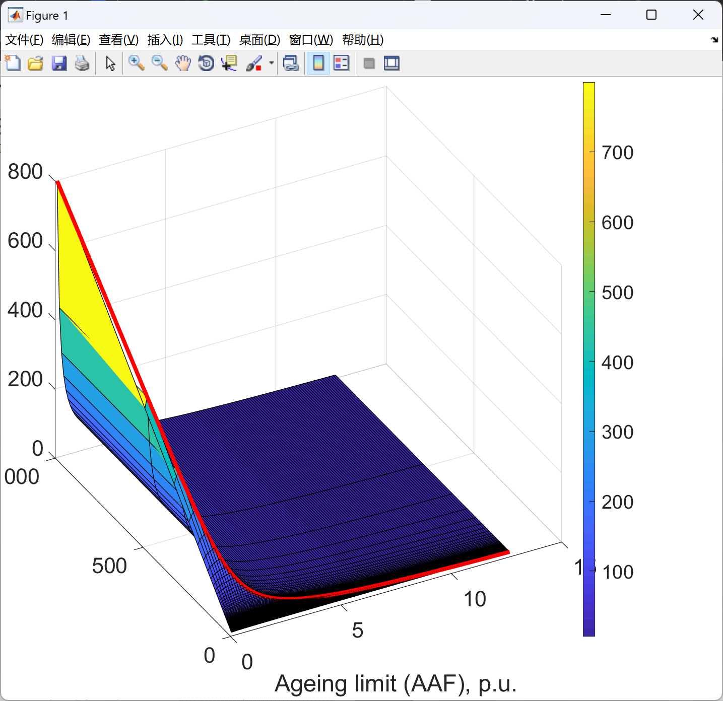
本文研究了柔性电力系统中变压器的最佳老化极限的选择。与类似研究不同,本文考虑了变压器的剩余日历寿命。此外,结果表明,对于相同的绝缘老化,可以通过变压器传输不同数量的能量。因此,本文将最大能量传输作为定义变压器(包括现有和新的变压器)最佳老化极限的标准。结果显示,变压器的最佳老化极限应该等于剩余绝缘寿命与剩余日历寿命之间的比率。此外,本文以新变压器的能量传输作为函数,考虑了各种老化极限和不同日历寿命持续时间。因此,如果系统操作员考虑变压器剩余绝缘寿命与剩余日历寿命之间的比率,老化极限的选择可能会不同于传统使用的(正常)老化极限。
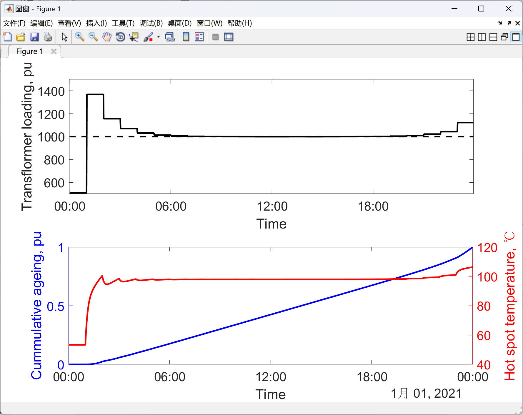
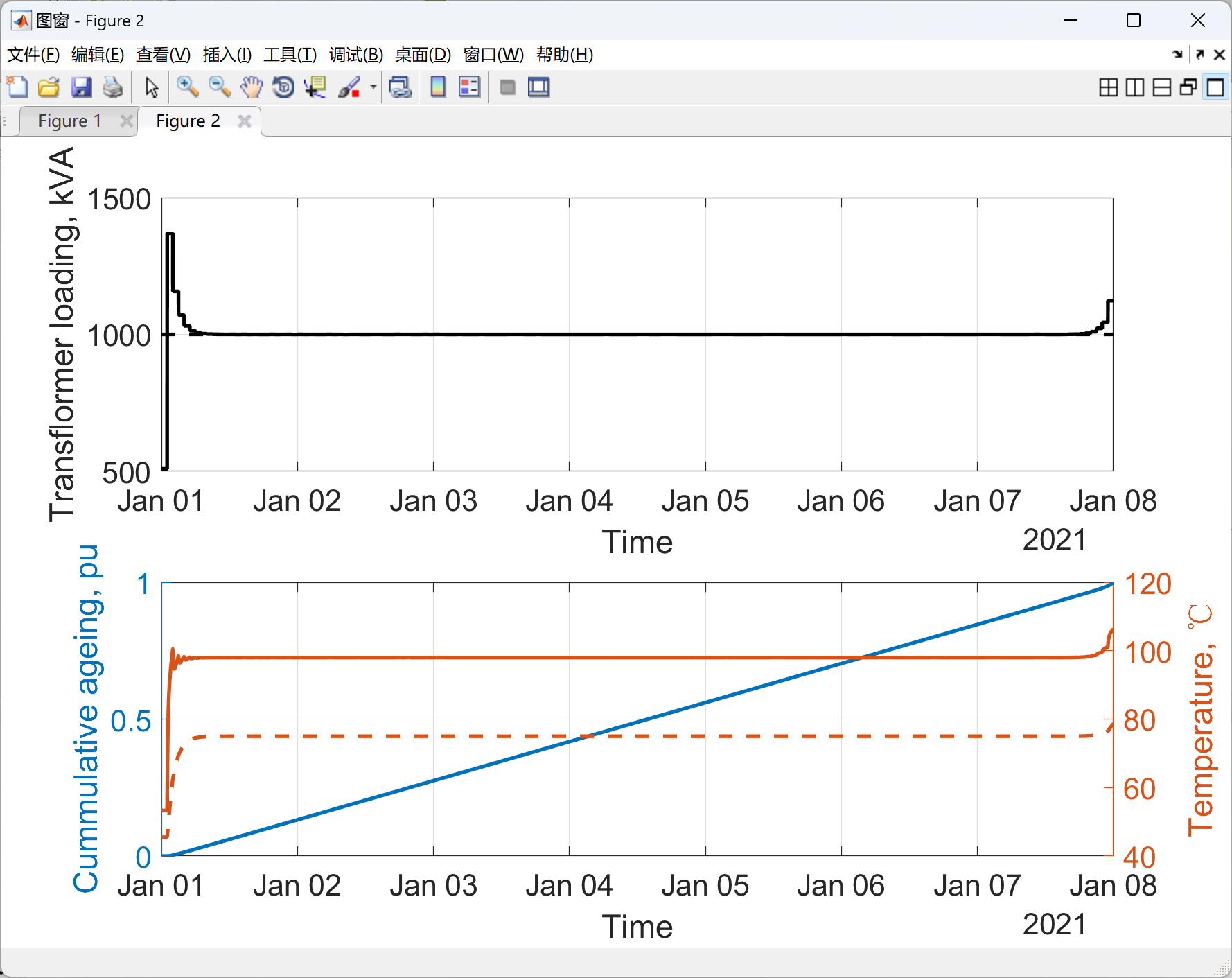
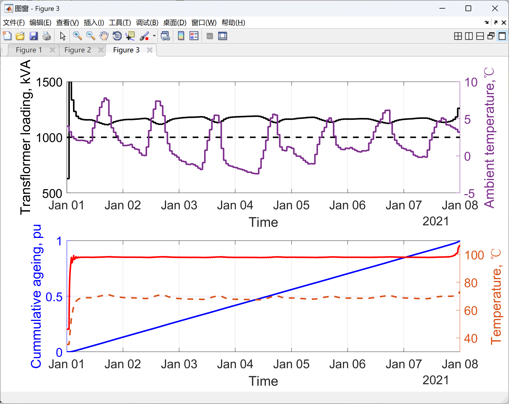
如今,能源行业正面临向脱碳电力系统过渡的能源转型。许多国家正在扩大可再生能源规模,以减少温室气体排放,但它们的电力网络面临着由拥挤、电压不稳定和谐波等因素引起的高压力。此外,供热和交通部门的持续电气化将进一步增加电力负荷,因此对电网基础设施造成压力。虽然分布式能源资源的份额持续快速增长,但电力网络无法以类似的速度加强。然而,随着电力系统变得前所未有地灵活,系统运营商迎来了新的机遇。例如,可控分布式发电、储能、需求侧管理和动态热负荷评估等技术可以减轻电力网络的压力。因此,在灵活电力系统中,系统运营商的挑战在于最大化电网基础设施的利用率。运营规划中考虑电网基础设施的利用率可以通过老化限制来实现。老化限制是一个综合约束条件,确保电力设备在可变温度下运行,其累积效应不超过规范损失寿命(LoL)。例如,在可变温度下运行的变压器的日常损失寿命不得超过如果同一变压器在恒定设计温度下运行时的损失寿命(通常为98ႏ RU)。系统运营商/研究人员的这种假设确保变压器可以按制造商预先定义的设计寿命全面运行。最近的研究证实,考虑到其剩余绝缘寿命,现有变压器的老化限制实际上可以提高到高于正常限制。事实上,由于长时间以来操作在正常老化限制以下,变压器仍具有显著的剩余寿命。图中展示了当变压器已经运行其设计寿命日历,但变压器仍保留一些绝缘资源以继续其运行的情况。
📚2 运行结果
 部分代码:
部分代码:
%% This script allows drawing the figure 6
% Use Section 1 to estimate the energy transfer as a function
% of ageing limit. (data generation)
% Otherwise, you can dircetly launch section 2 to construct the figure "ageing
% limit vs Energy transfer" from precalculated data.('ONAN_interm_results.mat')
% Section 3 draws the figure: Energy transfer as a function of time
% Section 4 prepares the data for Figure 8
%% Section 1: Generation of data
% Initial data
TIM=linspace(1,1440,1440)'; % time in minutes for 1 day
Temperature=-50:1:50; % Full range of ambient temperatures
Ageing_limit=0.1:0.1:12.7; % Range of Ageing_limits
AMB=linspace(20,20,24)'; % Fixed ambient temperature, hour time step
% Finding the energy transfer for each ageing limit
for i=1:length(Ageing_limit) % for ageing limit
% Solve the optimization problem for 1 day
[Energy_limit,HST_limit,AEQ_limit,TOT_limit,Energy]=optimal_energy_limitFig6(AMB,Ageing_limit(i));
% Save energy transfer. So far, units are pu*1min but later we will
% normalize them
Energy_result(i)=Energy;
% Energy limit (loading profile of transformer in pu)
PUL_result(1:1440,i)=Energy_limit;
% Loss of Life results
LoL_result(i)=AEQ_limit;
% caclulate the ageing acceleration factor (DL)
for m=1:length(HST_limit)
DL(m,:) = (2^((HST_limit(m)-98)/6));
end
% Calculate value of cummulated ageing at each moment
Current_ageing=0;
for j=1:length(DL)
Current_ageing(j)=Current_ageing(end)+DL(j);
end
%Save the result of cummulated ageing for given ageing limit (i)
Current_ageing_result(1:1440,i)=Current_ageing;
i % show the iteration
end
%% Section 2: Construct the figure ageing limit vs Energy transfer
clear;clc;close all
% Load the results from previous section
load('ONAN_interm_results.mat')
% Choose the calendar life left (see cases in Table 1 of the paper)
studied_case=1; % 1,2 or 3
if studied_case==1
% I case
calendar_time_left=50; % 50%
insulation_time_left=70; % 70%
elseif studied_case==2
% II case
calendar_time_left=50; % 50%
insulation_time_left=50; % 70%
elseif studied_case==3
% III case
calendar_time_left=50; % 50%
insulation_time_left=30; % 70%
else
error('Check the value of studied_case. It shoul be 1,2 or 3')
end
% Find the ratio (optimal ageing limit)
ratio=insulation_time_left/calendar_time_left;
% Find the calendar life in minutes of days
calendar_time_left_min=calendar_time_left*1440/100;
% Find the index which shows how fast insulation life left will be consumed at
% given ageing limit
for i=1:length(Ageing_limit)
index(i)=(insulation_time_left*1440/100)/Ageing_limit(i);
end
% Round the index to get an integer (approximation!)
index=round(index);
% Find time for which insulation resource can be used.
time_percent=(index./1440); % in pu
% Note that we calculate it relatively to 1 day 1440. Units are pu!
% Find how much energy is transfered for each ageing limit
for i=1:length(Ageing_limit)
if index(i)>calendar_time_left_min
ind=calendar_time_left_min;
else
ind=index(i);
end
Energy_day(i)=ind/calendar_time_left_min*sum(PUL_result(:,i));
end
% Energy_day=Energy_result;
% Normalize the energy transfer relatively to ageing limit =1 pu
Energy_day_percent=Energy_day/Energy_day(10)*100;
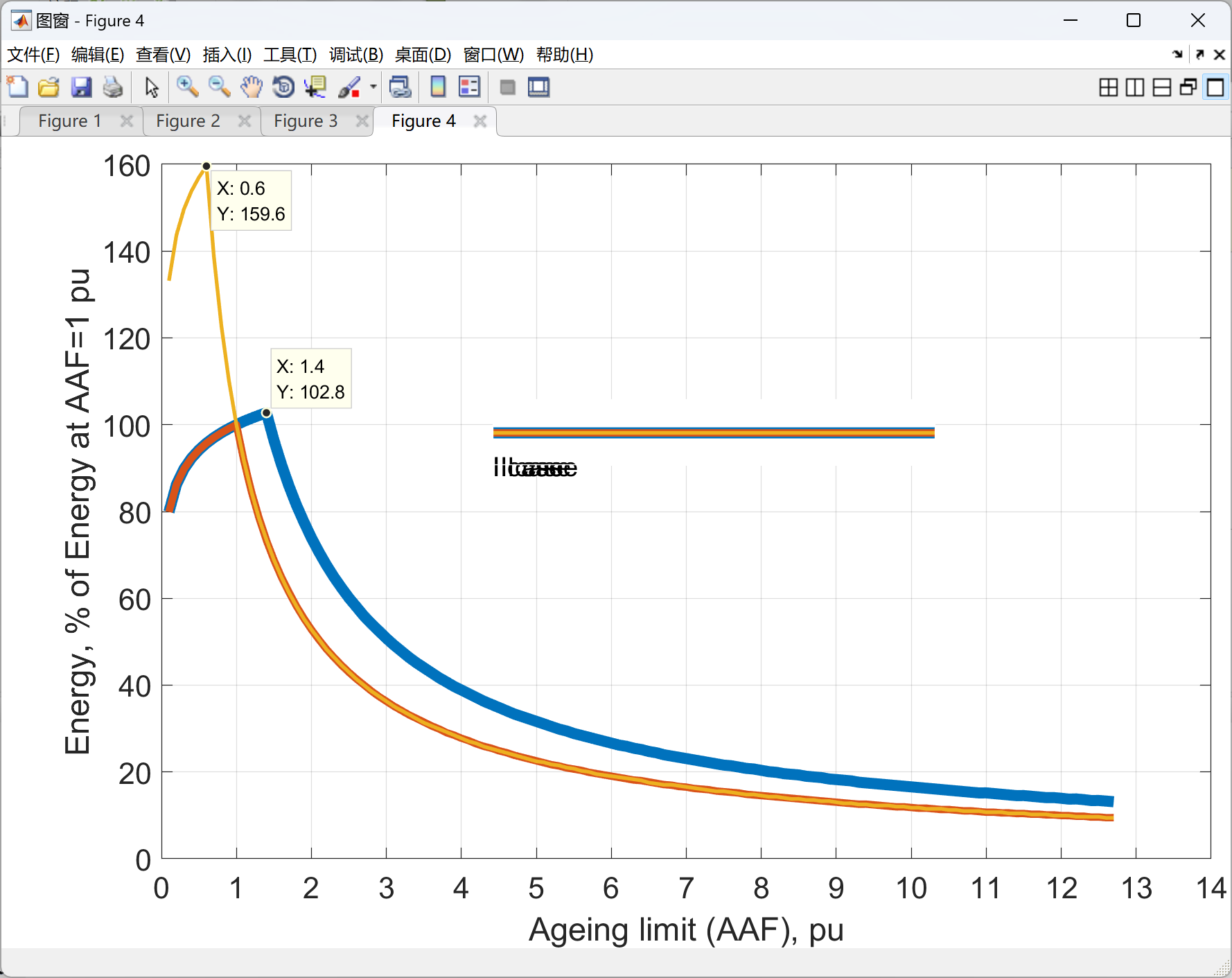
plot(Ageing_limit,Energy_day_percent)
ylabel('Energy, % of Energy at Ageing limit=1')
xlabel('Ageing limit(AAF), pu')
% time_percent=index/1440*100;
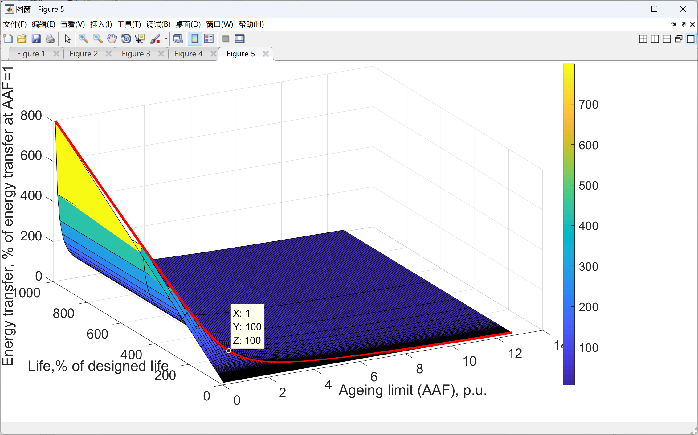
%% Section 3:Energy transfer as a function of time (additonal figure)
% Assumption: we assume that for each day the loading profile (and thus energy
% transfer) are the same. Thus, we can estimate how much energy can be
% transfered during the entire life if we multiply the energy trasnfer for
% 1 day on possible operation at given ageing limit (in per units!)
Energy_all_life=time_percent.*Energy_day;
% Normalize the energy transfer for each ageing limit (relatively to ageing
% limit = 1pu)
Energy_all_life=Energy_all_life./Energy_all_life(10)*100;
% Convert time_percent from pu into percent
time_percent=time_percent*100;
% Set the intitial position
start=[0 0];
figure % create the figure
hold on
🎉3 参考文献
文章中一些内容引自网络,会注明出处或引用为参考文献,难免有未尽之处,如有不妥,请随时联系删除。


 被折叠的 条评论
为什么被折叠?
被折叠的 条评论
为什么被折叠?
 到【灌水乐园】发言


