使用SSTL规范控制信号化交叉口研究（Matlab代码实现）

@橘柑橙柠桔柚

于 2024-06-30 09:22:20 发布

阅读量987

点赞数 32

文章标签： matlab 算法开发语言

本文链接：https://blog.csdn.net/weixin_61181717/article/details/140076545

版权

💥💥💞💞欢迎来到本博客❤️❤️💥💥

🏆博主优势：🌞🌞🌞博客内容尽量做到思维缜密，逻辑清晰，为了方便读者。

⛳️座右铭：行百里者，半于九十。

📋📋📋本文目录如下：🎁🎁🎁

目录

⛳️赠与读者

💥1 概述

📚2 运行结果

🎉3 参考文献

🌈4 Matlab代码实现

⛳️赠与读者

👨‍💻做科研，涉及到一个深在的思想系统，需要科研者逻辑缜密，踏实认真，但是不能只是努力，很多时候借力比努力更重要，然后还要有仰望星空的创新点和启发点。当哲学课上老师问你什么是科学，什么是电的时候，不要觉得这些问题搞笑。哲学是科学之母，哲学就是追究终极问题，寻找那些不言自明只有小孩子会问的但是你却回答不出来的问题。建议读者按目录次序逐一浏览，免得骤然跌入幽暗的迷宫找不到来时的路，它不足为你揭示全部问题的答案，但若能让人胸中升起一朵朵疑云，也未尝不会酿成晚霞斑斓的别一番景致，万一它居然给你带来了一场精神世界的苦雨，那就借机洗刷一下原来存放在那儿的“躺平”上的尘埃吧。

或许，雨过云收，神驰的天地更清朗.......🔎🔎🔎

💥1 概述

SSTL（Signalized Intersection Traffic Light）规范是一种用于控制信号化交叉口的标准规范，旨在提高交通效率、减少交通拥堵和事故发生率。研究SSTL规范在信号化交叉口的应用可以帮助交通管理部门优化交通信号控制方案，提高交通流量的运行效率。

研究SSTL规范控制信号化交叉口的具体内容可以包括以下几个方面：

1. 交通流量调查：通过对信号化交叉口周围交通流量的调查和分析，了解不同时间段的交通流量情况，为制定合理的信号控制方案提供数据支持。

2. 信号控制方案设计：根据交通流量调查结果和交叉口的特点，设计适合该交叉口的信号控制方案，包括信号灯的时序、相位设置等。

3. 仿真模拟分析：利用交通仿真软件对设计的信号控制方案进行模拟分析，评估其在不同交通流量条件下的效果，优化信号控制方案。

4. 实地验证与调整：在实际交通环境中对设计的信号控制方案进行验证，并根据实际效果进行调整和优化，确保交通信号控制的有效性和可靠性。

通过研究SSTL规范控制信号化交叉口，可以帮助交通管理部门更好地管理交通流量，提高交通运行效率，减少交通事故的发生率，改善城市交通环境。同时，也可以为未来智能交通系统的发展提供经验和借鉴。

SSTL规范是一种信号化交叉口控制系统，它采用了一种先进的信号控制技术，能够实现更高效、更安全的交通流动。研究SSTL规范在信号化交叉口的应用，可以帮助我们更好地理解这一系统的工作原理，优化控制策略，从而提高交通效率和减少交通事故的发生。

在研究SSTL规范控制信号化交叉口时，可以考虑以下几个方面：

1. 信号控制策略：研究不同的信号控制策略在不同交通流量情况下的效果，比较各种策略的优劣，寻找最优的控制方法。

2. 交通仿真模拟：使用交通仿真软件模拟不同交叉口场景下的交通流动情况，验证SSTL规范在实际环境中的有效性。

3. 交通数据分析：分析交通流量数据和信号控制数据，评估SSTL规范对交通流动的影响，找出可能存在的问题和改进的方向。

4. 现场实验：在实际交叉口进行现场实验，验证SSTL规范在实际环境中的效果，进一步完善控制策略。

通过以上方面的研究，可以深入了解SSTL规范在信号化交叉口的应用，为改善交通流动、提高交通安全性提供重要参考和支持。

📚2 运行结果

部分代码：

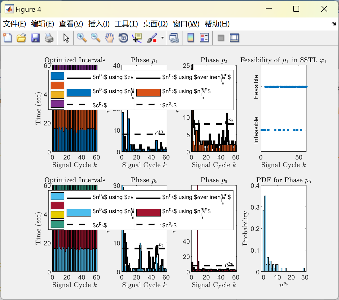
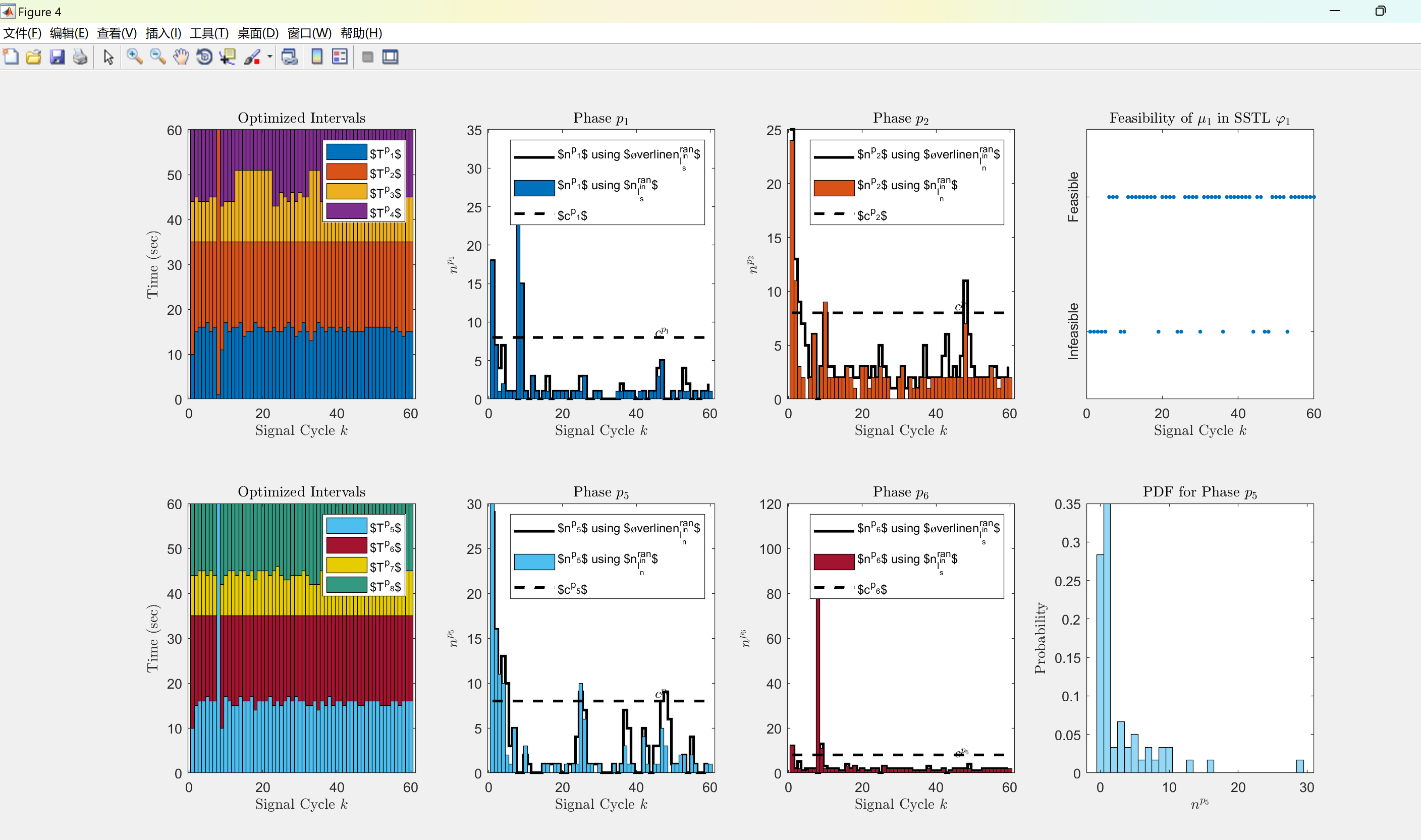
subplot(2,4,4); plot(SSTLPhi1FeasibilityUB,'.','MarkerSize',10);
title({'Feasibility of $\mu_{1}$ in SSTL $\varphi_{1}$'},'Interpreter','latex');
xlabel('Signal Cycle $k$','Interpreter','latex');
ylim([-0.5,1.5]);
yticks([0 1]);
yticklabels({'Infeasible','Feasible'});
ytickangle(90);

subplot(2,4,5); BarGraphp5p6p7p8 = bar(BarGraphMatrixp5p6p7p8, 'stacked','BarWidth',1);
BarGraphp5p6p7p8(1).FaceColor = [0.3010 0.7450 0.9330]; BarGraphp5p6p7p8(2).FaceColor = [0.6350 0.0780 0.1840];
BarGraphp5p6p7p8(3).FaceColor = [0.9 0.8 0]; BarGraphp5p6p7p8(4).FaceColor = [.2 .6 .5];
legend('$T^{p_{5}}$','$T^{p_{6}}$','$T^{p_{7}}$','$T^{p_{8}}$','Interpreter','latex');
title('Optimized Intervals','Interpreter','latex');
xlabel('Signal Cycle $k$','Interpreter','latex');
ylabel('Time (sec)','Interpreter','latex');

subplot(2,4,6); stairs(0.5:1:59.5,OptimalNNp5Green,'k','LineWidth',2);
hold on;
bar(ObservedNNp5Green,'FaceColor',[0.3010 0.7450 0.9330],'BarWidth',1);
title('Phase $p_{5}$','Interpreter','latex');
xlabel('Signal Cycle $k$','Interpreter','latex');
ylabel('$n^{p_{5}}$','Interpreter','latex');
ylim([0,30]);
hold on;
plot(NNp5GreenLimit*ones(1,NoSignalCycles),'--','Color','k','LineWidth',2);
legend('$n^{p_{5}}$ using $\overline{n}_{l_{n}^{in}}^{ran}$','$n^{p_{5}}$ using $n_{l_{n}^{in}}^{ran}$','$c^{p_{5}}$','Interpreter','latex');
text(45,NNp5GreenLimit+0.7,{'$c^{p_{5}}$'},'Interpreter','latex');

subplot(2,4,7); stairs(0.5:1:59.5,OptimalNSp6Green,'k','LineWidth',2);
hold on;
bar(ObservedNSp6Green,'FaceColor',[0.6350 0.0780 0.1840],'BarWidth',1);
title('Phase $p_{6}$','Interpreter','latex');
xlabel('Signal Cycle $k$','Interpreter','latex');
ylabel('$n^{p_{6}}$','Interpreter','latex');
%ylim([0, 10]);
hold on;
plot(NSp6GreenLimit*ones(1,NoSignalCycles),'--','Color','k','LineWidth',2);
legend('$n^{p_{6}}$ using $\overline{n}_{l_{s}^{in}}^{ran}$','$n^{p_{6}}$ using $n_{l_{s}^{in}}^{ran}$','$c^{p_{6}}$','Interpreter','latex');
text(45,NSp6GreenLimit+0.3,{'$c^{p_{6}}$'},'Interpreter','latex');

subplot(2,4,8); histogram(OptimalNNp5Green,'Normalization','probability','FaceColor',[0.3010 0.7450 0.9330]);
title('PDF for Phase $p_{5}$','Interpreter','latex');
xlabel('$n^{p_{5}}$','Interpreter','latex');
ylabel('Probability','Interpreter','latex');

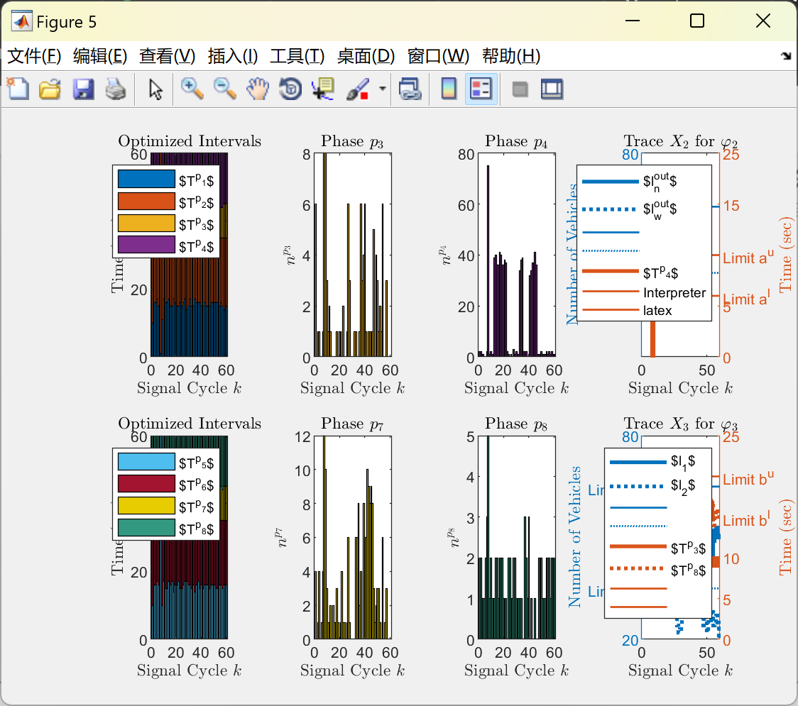
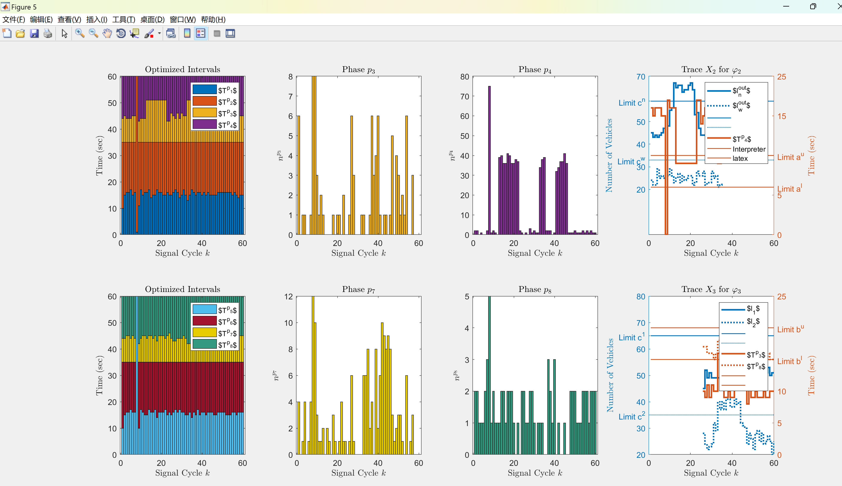
figure;
subplot(2,4,1); bar(BarGraphMatrixp1p2p3p4, 'stacked','BarWidth',1);
legend('$T^{p_{1}}$','$T^{p_{2}}$','$T^{p_{3}}$','$T^{p_{4}}$','Interpreter','latex');
title('Optimized Intervals','Interpreter','latex');
xlabel('Signal Cycle $k$','Interpreter','latex');
ylabel('Time (sec)','Interpreter','latex');

subplot(2,4,2); bar(ObservedNWp3Green,'FaceColor',[0.9290 0.6940 0.1250],'BarWidth',1);
title('Phase $p_{3}$','Interpreter','latex');
xlabel('Signal Cycle $k$','Interpreter','latex');
ylabel('$n^{p_{3}}$','Interpreter','latex');
ylim([0,8]);

subplot(2,4,3); bar(ObservedNEp4Green,'FaceColor',[0.4940 0.1840 0.5560],'BarWidth',1);
title('Phase $p_{4}$','Interpreter','latex');
xlabel('Signal Cycle $k$','Interpreter','latex');
ylabel('$n^{p_{4}}$','Interpreter','latex');
%ylim([0,40]);

subplot(2,4,4); yyaxis left;
stairs(N_downN(1,1:35),'LineWidth',2); hold on;
stairs(N_downW(1,1:35),':','LineWidth',2);
plot(59*ones(1,NoSignalCycles),'-','Color',[0 0.4470 0.7410],'LineWidth',1);
plot(33*ones(1,NoSignalCycles),':','Color',[0 0.4470 0.7410],'LineWidth',1);
legend('$l_{n}^{out}$','$l_{w}^{out}$','Interpreter','latex');
title({'Trace $X_{2}$ for $\varphi_{2}$'},'Interpreter','latex');
xlabel('Signal Cycle $k$','Interpreter','latex');
ylabel('Number of Vehicles','Interpreter','latex');
yticks([20 30 33 40 50 59 70 80]);
yticklabels({'20','30','Limit c^{w}','40','50','Limit c^{n}','70','80'});
yyaxis right;
stairs(BarGraphMatrixp1p2p3p4(1:35,4),'LineWidth',2);
plot(10*ones(1,NoSignalCycles),'-','Color',[0.8500 0.3250 0.0980],'LineWidth',1);
plot(6*ones(1,NoSignalCycles),'-','Color',[0.8500 0.3250 0.0980],'LineWidth',1);
legend('$l_{n}^{out}$','$l_{w}^{out}$','','','$T^{p_{4}}$','Interpreter','latex');
ylabel('Time (sec)','Interpreter','latex');
yticks([0 5 6 10 15 20]);
yticklabels({'0','5','Limit a^{l}','Limit a^{u}','15','25'});
xlim([0,60]);
ylim([0,20]);

subplot(2,4,5); BarGraphp5p6p7p8 = bar(BarGraphMatrixp5p6p7p8,'stacked','BarWidth',1);
BarGraphp5p6p7p8(1).FaceColor = [0.3010 0.7450 0.9330]; BarGraphp5p6p7p8(2).FaceColor = [0.6350 0.0780 0.1840];
BarGraphp5p6p7p8(3).FaceColor = [0.9 0.8 0]; BarGraphp5p6p7p8(4).FaceColor = [.2 .6 .5];
legend('$T^{p_{5}}$','$T^{p_{6}}$','$T^{p_{7}}$','$T^{p_{8}}$','Interpreter','latex');
title('Optimized Intervals','Interpreter','latex');
xlabel('Signal Cycle $k$','Interpreter','latex');
ylabel('Time (sec)','Interpreter','latex');

subplot(2,4,6); bar(ObservedNEp7Green,'FaceColor',[0.9 0.8 0],'BarWidth',1);
title('Phase $p_{7}$','Interpreter','latex');
xlabel('Signal Cycle $k$','Interpreter','latex');
ylabel('$n^{p_{7}}$','Interpreter','latex');
ylim([0,12]);

subplot(2,4,7); bar(ObservedNWp8Green,'FaceColor',[.2 .6 .5],'BarWidth',1);
title('Phase $p_{8}$','Interpreter','latex');
xlabel('Signal Cycle $k$','Interpreter','latex');
ylabel('$n^{p_{8}}$','Interpreter','latex');
ylim([0,5]);

subplot(2,4,8); yyaxis left;
stairs((26:1:60),N_upN(1,26:end),'LineWidth',2); hold on;
stairs((26:1:60),N_upS(1,26:end),':','LineWidth',2);
plot(65*ones(1,NoSignalCycles),'-','Color',[0 0.4470 0.7410],'LineWidth',1);
plot(35*ones(1,NoSignalCycles),':','Color',[0 0.4470 0.7410],'LineWidth',1);
title({'Trace $X_{3}$ for $\varphi_{3}$'},'Interpreter','latex');
xlabel('Signal Cycle $k$','Interpreter','latex');
ylabel('Number of Vehicles','Interpreter','latex');
yticks([20 30 35 40 50 60 65 70 80]);
yticklabels({'20','30','Limit c^{2}','40','50','60','Limit c^{1}','70','80'});
yyaxis right;
stairs((26:1:60),BarGraphMatrixp1p2p3p4(26:end,3),'LineWidth',2);
stairs((26:1:60),BarGraphMatrixp5p6p7p8(26:end,4),':','LineWidth',2);
plot(15*ones(1,NoSignalCycles),'-','Color',[0.8500 0.3250 0.0980],'LineWidth',1);
plot(20*ones(1,NoSignalCycles),'-','Color',[0.8500 0.3250 0.0980],'LineWidth',1);
legend('$l_{1}$','$l_{2}$','','','$T^{p_{3}}$','$T^{p_{8}}$','','','Interpreter','latex');
ylabel('Time (sec)','Interpreter','latex');
yticks([0 5 10 15 20 25]);
yticklabels({'0','5','10','Limit b^{l}','Limit b^{u}','25'});
ylim([0,25]);

🎉3 参考文献

文章中一些内容引自网络，会注明出处或引用为参考文献，难免有未尽之处，如有不妥，请随时联系删除。

[1]张海良.DDR SDRAM物理层的SSTL接口电路设计[D].哈尔滨工业大学[2024-05-07].DOI:CNKI:CDMD:2.1011.261573.

[2]朱胜华,胡福乔,施鹏飞.平面交叉路口信号灯自动配时方案的优化算法[J].交通信息与安全, 2002, 020(004):3-8.DOI:10.3963/j.issn.1674-4861.2002.04.001.

[3]袁二明,涂奉生,蔡小强.基于混合整数规划的相邻交叉路口信号协调控制[J].系统工程, 2006, 24(8):6.DOI:10.3969/j.issn.1001-4098.2006.08.007.

[4]郝林倩.基于多目标优化算法的交叉路口信号灯配时模型研究[J].智能计算机与应用, 2021.DOI:10.3969/j.issn.2095-2163.2021.03.033.

🌈4 Matlab代码实现

@橘柑橙柠桔柚

关注

32
点赞
踩
26

收藏

觉得还不错? 一键收藏
0
评论
使用SSTL规范控制信号化交叉口研究（Matlab代码实现）

SSTL（Signalized Intersection Traffic Light）规范是一种用于控制信号化交叉口的标准规范，旨在提高交通效率、减少交通拥堵和事故发生率。研究SSTL规范在信号化交叉口的应用可以帮助交通管理部门优化交通信号控制方案，提高交通流量的运行效率。研究SSTL规范控制信号化交叉口的具体内容可以包括以下几个方面：1. 交通流量调查：通过对信号化交叉口周围交通流量的调查和分析，了解不同时间段的交通流量情况，为制定合理的信号控制方案提供数据支持。
复制链接

扫一扫