


前言
本案例使用LightGBM算法对餐厅营收训练数据进行训练,并对测试数据进行预测,之后通过调参优化模型。结果表明,该算法对数据有良好的预测效果,调参之后模型得到优化。
数据了解
这里分为两个文件,一个是训练数据集restaurant_data_train.csv,一个是测试数据集restaurant_data_test.csv,我们将其导入,并一步步了解其数据情况。这里跳过一些简单的数据规模介绍(大致情况是:训练集有137条数据、43个特征;测试集有100000条数据、42个特征),代码及数据情况如下:
import pandas as pd
import numpy as np
import matplotlib.pyplot as plt
import seaborn as sns
from sklearn.preprocessing import LabelEncoder
from sklearn.model_selection import train_test_split, RandomizedSearchCV
from sklearn.metrics import mean_absolute_error, r2_score, mean_squared_log_error
import lightgbm as lgb
import warnings
warnings.filterwarnings('ignore')
# 导入数据
df_train = pd.read_csv("data/restaurant_data_train.csv")
df_test = pd.read_csv("data/restaurant_data_test.csv")
print(df_train.info())
print(df_train.describe())
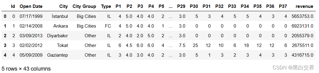
print(df_train.head())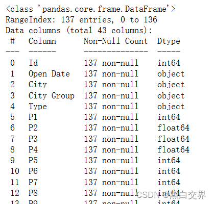
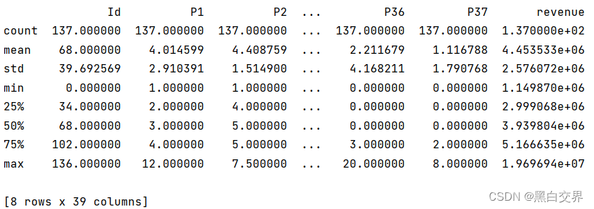
其中P1到P37为保密特征,所以特征名称用编号代替。这里由于开业时间、所属城市、城市类型、餐饮类型几个字段都是类型字段而非数值型字段,所以不在describe范围内。
接下来是对特征字段的进一步认识,用绘图的方式了解字段。(与建模无关,不感兴趣可以直接跳过)
# city 数据统计分布
plt.figure(figsize=(12,8))
sns.countplot(x='City',data=df_train)
plt.xticks(rotation='vertical') # 横轴数值改变方向
plt.show()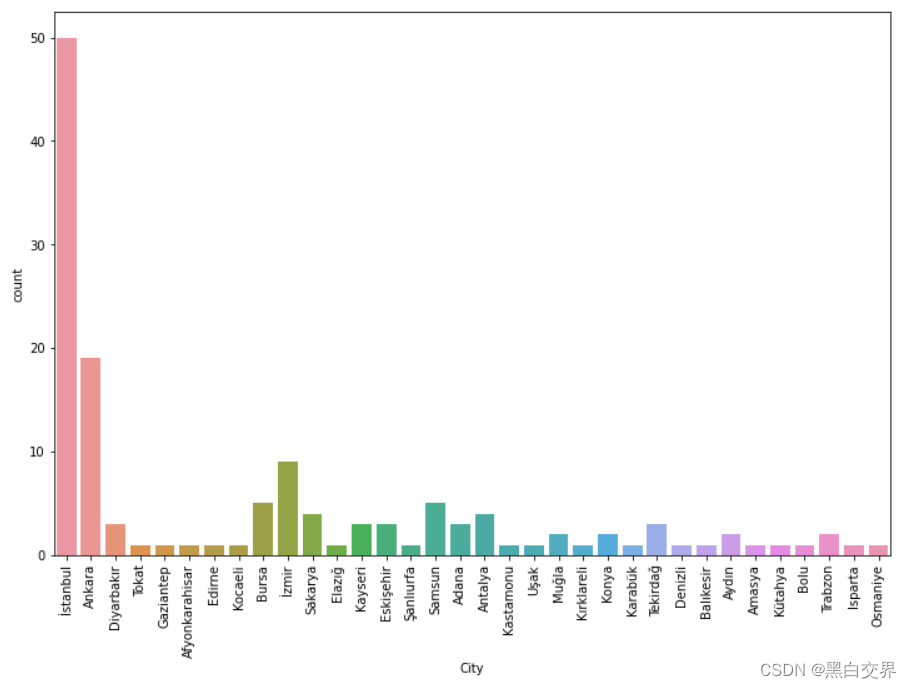
istanbul的餐厅数量最多,其次是Ankara
# City Group 分析
plt.figure(figsize=(12,8))
sns.countplot(x='City Group', data=df_train)
plt.show()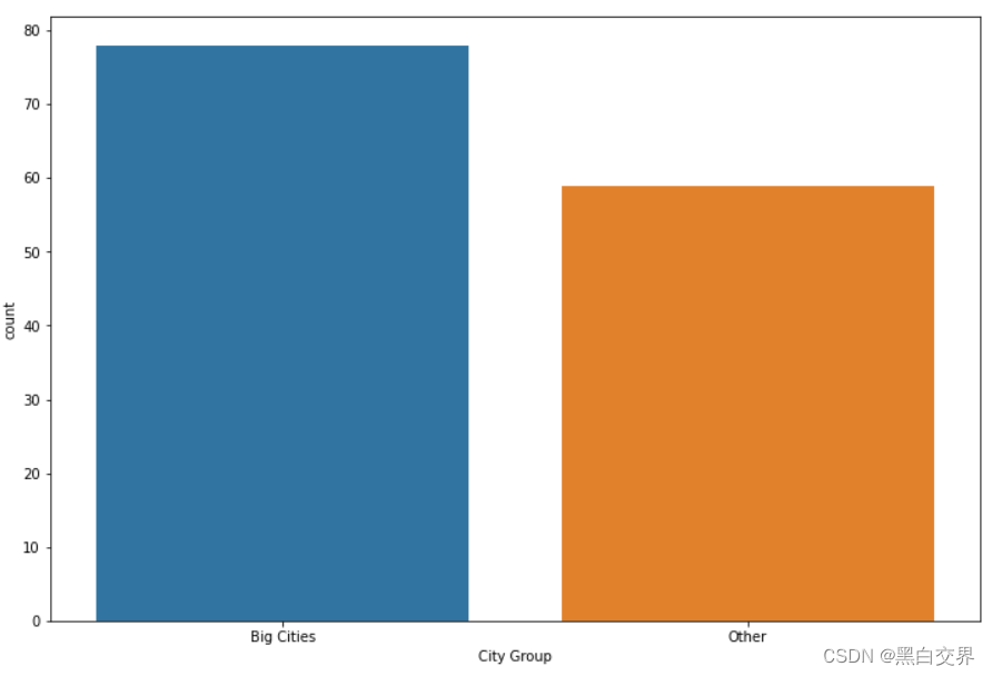
78家餐厅在大城市,59家餐厅在其它城市
# Type 餐厅类型分析
plt.figure(figsize=(12,8))
sns.countplot(x='Type', data=df_train)
plt.show()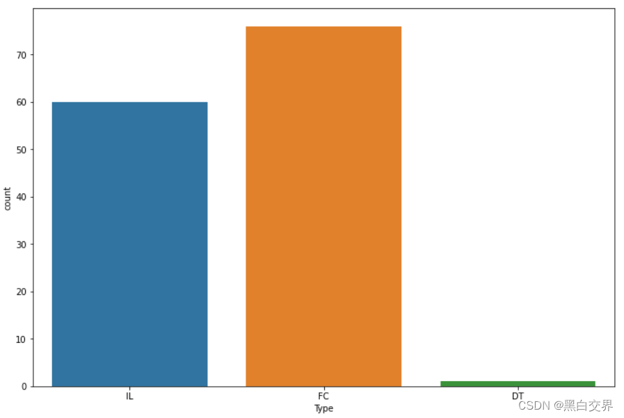
- 一共有3种类型的餐厅,FC: Food Court 美食街, IL: Inline 堂食, DT: Drive Thru 快餐(得来速)
- IL餐厅数量60家,FC餐厅数量76家,DT餐厅数量1家
# 分析 City 与 revenue 之间的关系
plt.figure(figsize=(12,8))
sns.boxplot(x='City', y='revenue', data=df_train) # 箱线图
plt.xlabel('cities', fontsize=12) # 设置横轴
plt.ylabel('revenue', fontsize=12) # 设置纵轴
plt.title("Relation between cities and revenue") # 标题
plt.xticks(rotation=90) # 旋转90度
plt.show()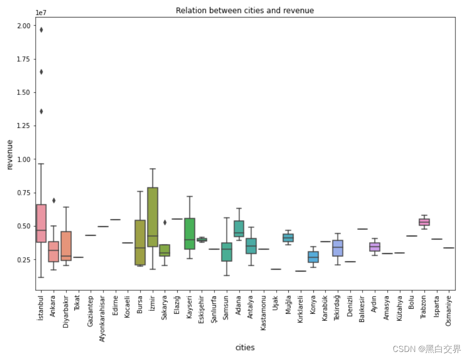
- 城市izmir的收益最高,其次是城市istanbul;
- 在城市istanbul出现了多处异常值,后续需要进行清理;
- 在城市Ankara和Sakarya也出现了异常值,不过数量很少,影响不大;
- 在城市Trabzon开的餐厅数量少,但是收益非常好。
# 分析 Type 与 revenue 之间的联系
plt.figure(figsize=(16,8))
sns.scatterplot(x='Type', y='revenue', data=df_train) # 散点图
plt.xlabel("City types",fontsize=12) # 横轴
plt.ylabel("Revenue", fontsize=12) # 纵轴
plt.show()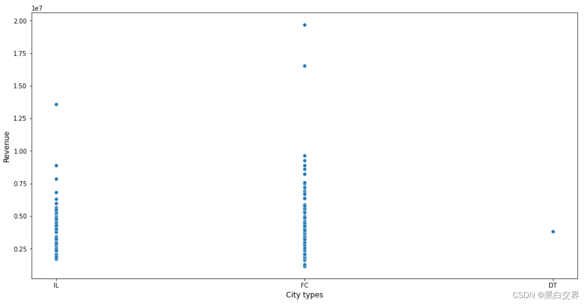
- 餐厅类型是FC,收益最高,也存在少数异常值;
- 其次是餐厅类型IL的收益高,少数异常值;
- 最后一个餐厅是DT类型,收益相比于其它两种类型处于居中状态
# 分析特征P之间的关系
plt.figure(figsize=(16,8))
feature_df = df_train.iloc[:, 5:] # 筛选出P特征所在列
col_names = feature_df.columns[:-1]
sns.pairplot(data=feature_df, x_vars=col_names)
plt.show()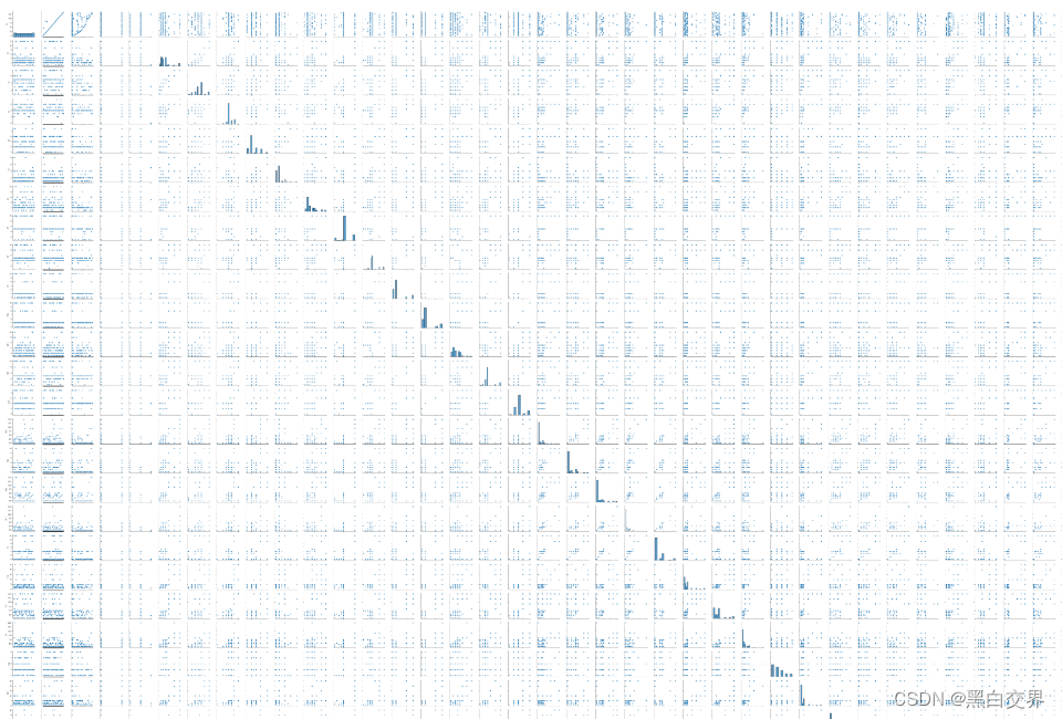
(这个图片较大,画图时间较长,实践运行时不建议show出来)
# 数据关系热图
cr = df_train.corr()
plt.figure(figsize=(18, 10))
sns.heatmap(cr, annot=False)
plt.show()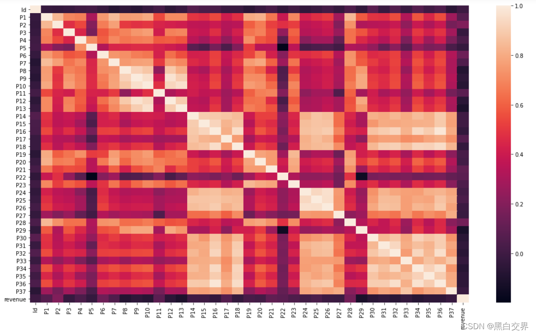
数据预处理
这里主要是对日期类型数据进行转化。并且通过对数据的解读可知营收一列存在异常值,我们将其去除。
# 日期类型转换
df_train['Open Date'] = pd.to_datetime(df_train['Open Date'])
df_test['Open Date'] = pd.to_datetime(df_train['Open Date'])
# 去除Revenue中的异常值
df_train = df_train[df_train['revenue'] < 1.1 * 1e7]  # 将大于11000000
# print(df_train.shape)
特征工程
这里主要是将分类型数据转化为数值型数据。
# 分类类型进行转换
def label_encoding(df, cols):
    for col in cols:
        le = LabelEncoder()
        df[col] = le.fit_transform(df[col])
    return df
category_cols = df_train.columns[df_train.dtypes == 'object'] # 筛选出分类类型的字段
df_train = label_encoding(df_train, category_cols)
df_test = label_encoding(df_test, category_cols)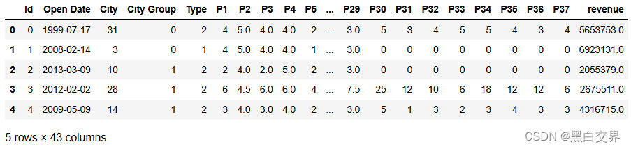
模型构建
初步构建LightGBM模型,在测试集上验证模型性能。
# 模型训练、验证
x = df_train.drop(['Id', 'Open Date','revenue'], axis=1)  # 特征集
y = df_train['revenue']  # 标签集
x_train, x_test, y_train, y_test = train_test_split(x.values, y.values, test_size=0.2, random_state=666)
model = lgb.LGBMRegressor()
model.fit(x_train, y_train)
# 验证
y_pred = model.predict(x_test)
MAE = mean_absolute_error(y_test, y_pred)
print(MAE)
MSE = mean_squared_log_error(y_test, y_pred)
print(MSE)
输出结果为:
MAE:1548178.1443002778;MSE:0.1895054945848149
# 测试
df_test = df_test.drop(['Id', 'Open Date'], axis=1)
preds_value = model.predict(df_test)
pred_df = pd.DataFrame(preds_value, columns=['pred_revenue'])
df_test = pd.concat([df_test, pred_df], axis=1)  # 将预测结果拼接到test中
print(df_test.head())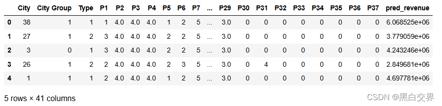
# 预测结果可视化
plt.figure(figsize=(16,8))
plt.hist(df_test['pred_revenue'], bins=30, edgecolor='black')
plt.title('Distribution of pred_revenue')
plt.xlabel('pred_revenue')
plt.ylabel('Frequency')
plt.grid(True)
plt.show()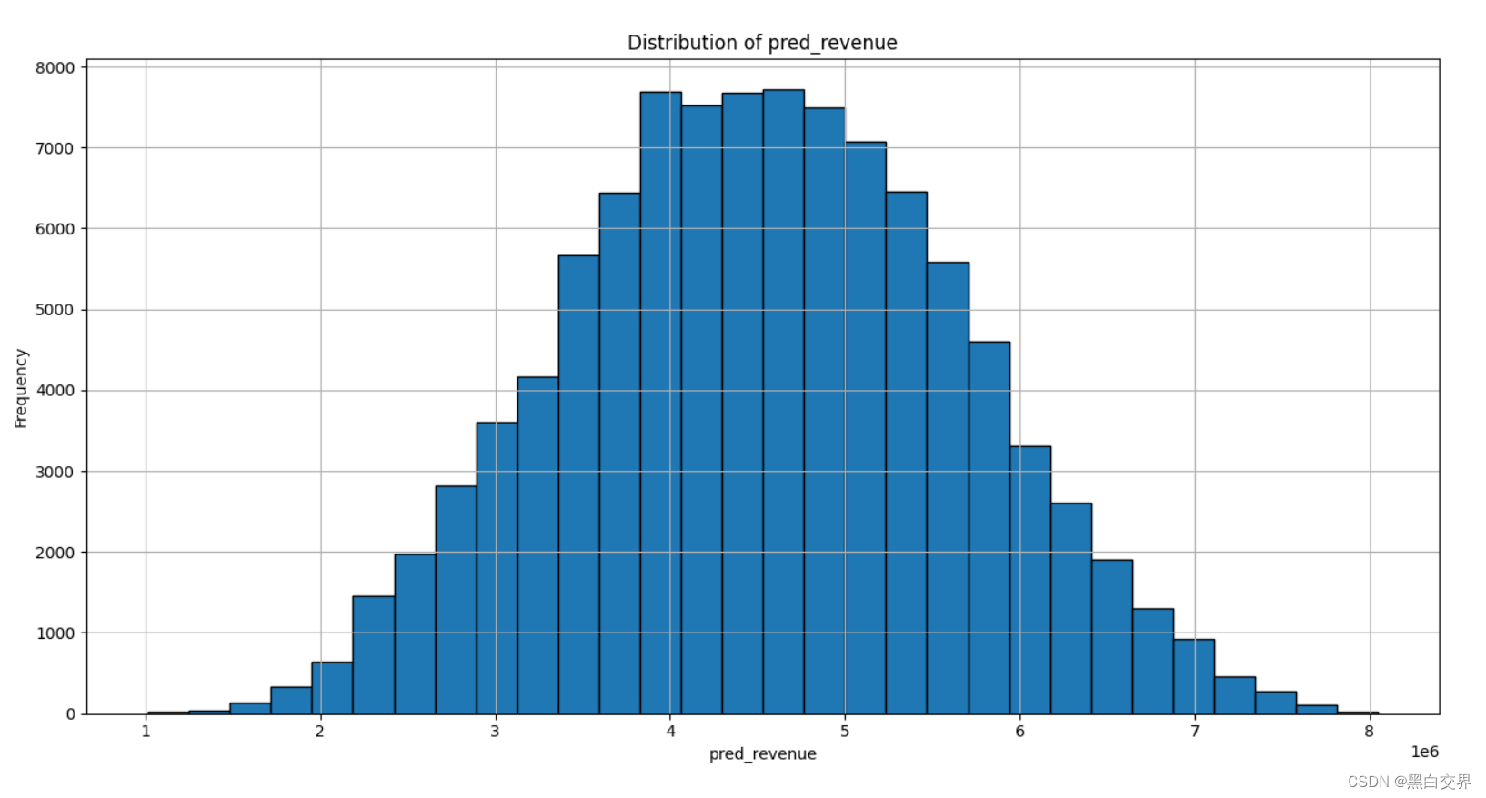
从上图可以看出,预测值基本符合正态分布。
模型优化
接下类使用交叉验证的方式训练模型来寻找最优超参数集合,并得出优化的LightGBM模型,将优化前后的预测能力进行对比。
# 默认参数
fit_params = {
'early_stopping_rounds' : 30,
'eval_metric' : 'regressor',
'eval_set' : [(x_test, y_test)],
'eval_names' : ['valid'],
'verbose' : 0,
'categorical_feature' : 'auto'
}
# 搜索超参数
params_test = {
'learning_rate': [0.01, 0.02, 0.03, 0.05, 0.07, 0.1, 0.2, 0.3, 0.4], # 学习率
'n_estimators': np.arange(100, 500, 50), # 树模型
'num_leaves': np.arange(10, 50), # 叶子数
'min_child_samples': np.arange(100, 500, 50), # 最小子节点样本数
'max_depth': np.arange(1, 10), # 树的深度
}
n_iter = 50 # 循环50轮
# 初始化模型
model = lgb.LGBMRegressor(random_state=666, n_jobs=-1)
# 网格搜索
grid_search = RandomizedSearchCV(estimator=model,
param_distributions = params_test,
n_iter = n_iter,
scoring = 'neg_mean_absolute_error',
random_state = 666,
verbose = True,
n_jobs = -1)
# 训练
grid_search.fit(x_train, y_train, **fit_params)
# 输出
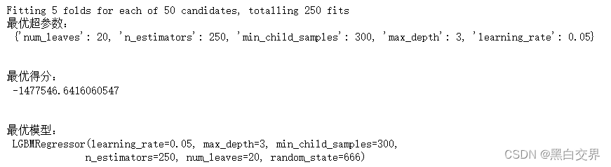
print("最优超参数:\n", grid_search.best_params_)
print("最优得分:\n", grid_search.best_score_)
print("最优模型:\n", grid_search.best_estimator_)得到最优超参数以及最优模型如下:
# 新模型预测
best_model = grid_search.best_estimator_
y_pred = best_model.predict(x_test)
MAE_02 = mean_absolute_error(y_test, y_pred)
print(MAE_02)
MSE_02 = mean_squared_log_error(y_test, y_pred)
print(MSE_02)
输出结果为:
MAE_02:1123810.7653167185;MSE_02:0.13562322991540746
可以看出两者都要比模型优化前要小,模型优化有效。
完整代码
import pandas as pd
import numpy as np
import matplotlib.pyplot as plt
import seaborn as sns
from sklearn.preprocessing import LabelEncoder
from sklearn.model_selection import train_test_split, RandomizedSearchCV
from sklearn.metrics import mean_absolute_error, r2_score, mean_squared_log_error
import lightgbm as lgb
import warnings
warnings.filterwarnings('ignore')

# 导入数据
df_train = pd.read_csv("data/restaurant_data_train.csv")
df_test = pd.read_csv("data/restaurant_data_test.csv")
# print(df_train.info()) # 数据信息
# print(df_train.describe())

### 数据了解 ###
plt.figure(figsize=(12,8))
sns.countplot(x='City',data=df_train)
plt.xticks(rotation='vertical') # 横轴数值改变方向
# plt.show()

# print("根据city group分组统计:\n", df_train['City Group'].value_counts())

plt.figure(figsize=(12,8))
sns.countplot(x='City Group', data=df_train)
# plt.show()

# print("根据Type分组统计:\n", df_train['Type'].value_counts())

plt.figure(figsize=(12,8))
sns.countplot(x='Type', data=df_train)
# plt.show()

# 分析 City 与 revenue 之间的关系
plt.figure(figsize=(12,8))
sns.boxplot(x='City', y='revenue', data=df_train) # 箱线图
plt.xlabel('cities', fontsize=12) # 设置横轴
plt.ylabel('revenue', fontsize=12) # 设置纵轴
plt.title("Relation between cities and revenue") # 标题
plt.xticks(rotation=90) # 旋转90度
# plt.show()

# 分析 Type 与 revenue 之间的联系
plt.figure(figsize=(16,8))
sns.scatterplot(x='Type', y='revenue', data=df_train) # 散点图
plt.xlabel("City types",fontsize=12) # 横轴
plt.ylabel("Revenue", fontsize=12) # 纵轴
# plt.show()

# 分析特征P之间的关系
plt.figure(figsize=(16,8))
feature_df = df_train.iloc[:, 5:]
col_names = feature_df.columns[:-1]
sns.pairplot(data=feature_df, x_vars=col_names)
# plt.show()

# 数据关系热图
cr = df_train.corr()
plt.figure(figsize=(18, 10))
sns.heatmap(cr, annot=False)
# plt.show()

### 数据预处理 ###
# 日期类型转换
df_train['Open Date'] = pd.to_datetime(df_train['Open Date'])
df_test['Open Date'] = pd.to_datetime(df_train['Open Date'])
# 去除Revenue中的异常值
df_train = df_train[df_train['revenue'] < 1.1 * 1e7] # 将大于 11000000
# print(df_train.shape)

### 特征工程 ###
# 分类类型进行转换
def label_encoding(df, cols):
    for col in cols:
        le = LabelEncoder()
        df[col] = le.fit_transform(df[col])
    return df
category_cols = df_train.columns[df_train.dtypes == 'object'] # 筛选出分类类型的字段
df_train = label_encoding(df_train, category_cols)
df_test = label_encoding(df_test, category_cols)

### 模型训练、验证 ###
x = df_train.drop(['Id', 'Open Date','revenue'], axis=1)  # 特征集
y = df_train['revenue']  # 标签集
x_train, x_test, y_train, y_test = train_test_split(x.values, y.values, test_size=0.2, random_state=666)
model = lgb.LGBMRegressor()
model.fit(x_train, y_train)
# 验证
y_pred = model.predict(x_test)
MAE = mean_absolute_error(y_test, y_pred)
print(MAE)
MSE = mean_squared_log_error(y_test, y_pred)
print(MSE)
# 测试
df_test = df_test.drop(['Id', 'Open Date'], axis=1)
preds_value = model.predict(df_test)
pred_df = pd.DataFrame(preds_value, columns=['pred_revenue'])
df_test = pd.concat([df_test, pred_df], axis=1)  # 将预测结果拼接到test中
print(df_test.head())
# 预测结果可视化
plt.figure(figsize=(16,8))
plt.hist(df_test['pred_revenue'], bins=30, edgecolor='black')
plt.title('Distribution of pred_revenue')
plt.xlabel('pred_revenue')
plt.ylabel('Frequency')
plt.grid(True)
plt.show()

### 交叉验证,寻找最优超参数 ###
# 默认参数
fit_params = {
    'early_stopping_rounds' : 30,
    'eval_metric' : 'regressor',
    'eval_set' : [(x_test, y_test)],
    'eval_names' : ['valid'],
    'verbose' : 0,
    'categorical_feature' : 'auto'
}

# 搜索超参数
params_test = {
    'learning_rate': [0.01, 0.02, 0.03, 0.05, 0.07, 0.1, 0.2, 0.3, 0.4], # 学习率
    'n_estimators': np.arange(100, 500, 50), # 树模型
    'num_leaves': np.arange(10, 50), # 叶子数
    'min_child_samples': np.arange(100, 500, 50), # 最小子节点样本数
    'max_depth': np.arange(1, 10), # 树的深度
}

n_iter = 50 # 循环50轮

# 初始化模型
model = lgb.LGBMRegressor(random_state=666, n_jobs=-1)

# 网格搜索
grid_search = RandomizedSearchCV(estimator=model,
                                 param_distributions = params_test,
                                 n_iter = n_iter,
                                 scoring = 'neg_mean_absolute_error',
                                 random_state = 666,
                                 verbose = True,
                                 n_jobs = -1)
# 训练
grid_search.fit(x_train, y_train, **fit_params)
# 输出
print("最优超参数:\n", grid_search.best_params_)
print("最优得分:\n", grid_search.best_score_)
print("最优模型:\n", grid_search.best_estimator_)

# 新模型预测
best_model = grid_search.best_estimator_
y_pred = best_model.predict(x_test)
MAE_02 = mean_absolute_error(y_test, y_pred)
print(MAE_02)
MSE_02 = mean_squared_log_error(y_test, y_pred)
print(MSE_02)
缺点与不足:本次案例的训练数据量太小,LightGBM应用于大规模数据集才能更好的生效。
本文参考B站唐国梁Tommy的讲解视频


 被折叠的 条评论
为什么被折叠?
被折叠的 条评论
为什么被折叠?
 到【灌水乐园】发言


