NNDL 实验五前馈神经网络（3）鸢尾花分类

最新推荐文章于 2024-04-24 11:55:13 发布

红肚兜

最新推荐文章于 2024-04-24 11:55:13 发布

阅读量822

点赞数 3

文章标签：神经网络分类算法

本文链接：https://blog.csdn.net/weixin_63539289/article/details/127309066

版权

深入研究鸢尾花数据集

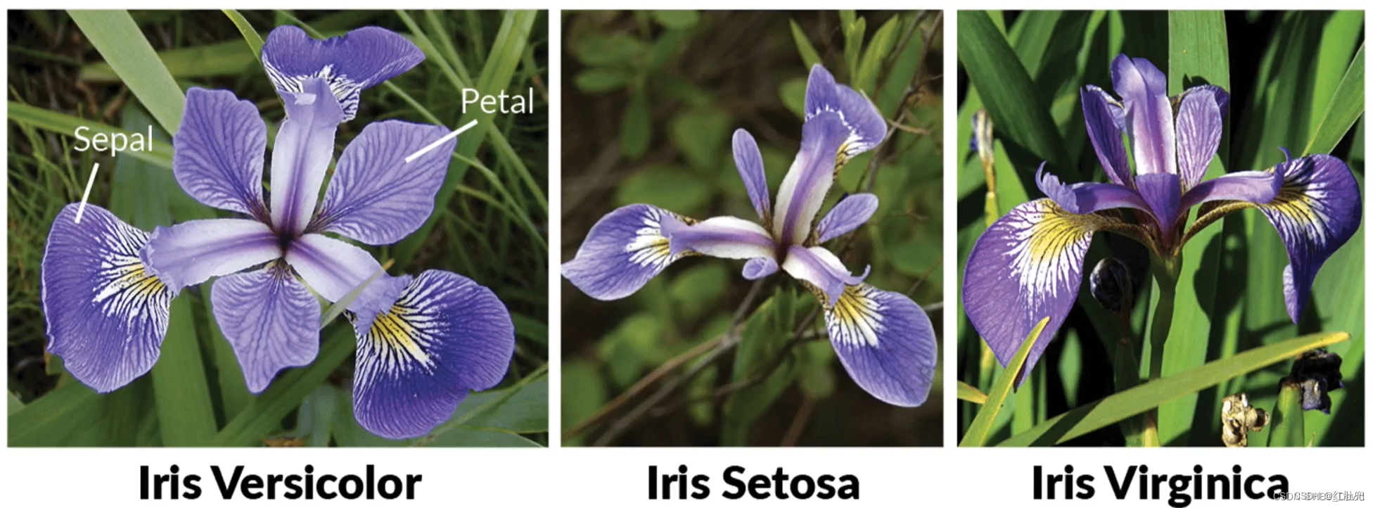
鸢尾花数据集也就是iris数据集，是一个非常经典的数据集，各路大神一定并不陌生。这次实验我们就以此为实验来源，对鸢尾花进行分类。为防止有的同学不知道这个数据集，下面给出这个数据集以及可视化深入了解一下。
在这里插入图片描述

Id,SepalLengthCm,SepalWidthCm,PetalLengthCm,PetalWidthCm,Species
1,5.1,3.5,1.4,0.2,Iris-setosa
2,4.9,3.0,1.4,0.2,Iris-setosa
3,4.7,3.2,1.3,0.2,Iris-setosa
4,4.6,3.1,1.5,0.2,Iris-setosa
5,5.0,3.6,1.4,0.2,Iris-setosa
6,5.4,3.9,1.7,0.4,Iris-setosa
7,4.6,3.4,1.4,0.3,Iris-setosa
8,5.0,3.4,1.5,0.2,Iris-setosa
9,4.4,2.9,1.4,0.2,Iris-setosa
10,4.9,3.1,1.5,0.1,Iris-setosa
11,5.4,3.7,1.5,0.2,Iris-setosa
12,4.8,3.4,1.6,0.2,Iris-setosa
13,4.8,3.0,1.4,0.1,Iris-setosa
14,4.3,3.0,1.1,0.1,Iris-setosa
15,5.8,4.0,1.2,0.2,Iris-setosa
16,5.7,4.4,1.5,0.4,Iris-setosa
17,5.4,3.9,1.3,0.4,Iris-setosa
18,5.1,3.5,1.4,0.3,Iris-setosa
19,5.7,3.8,1.7,0.3,Iris-setosa
20,5.1,3.8,1.5,0.3,Iris-setosa
21,5.4,3.4,1.7,0.2,Iris-setosa
22,5.1,3.7,1.5,0.4,Iris-setosa
23,4.6,3.6,1.0,0.2,Iris-setosa
24,5.1,3.3,1.7,0.5,Iris-setosa
25,4.8,3.4,1.9,0.2,Iris-setosa
26,5.0,3.0,1.6,0.2,Iris-setosa
27,5.0,3.4,1.6,0.4,Iris-setosa
28,5.2,3.5,1.5,0.2,Iris-setosa
29,5.2,3.4,1.4,0.2,Iris-setosa
30,4.7,3.2,1.6,0.2,Iris-setosa
31,4.8,3.1,1.6,0.2,Iris-setosa
32,5.4,3.4,1.5,0.4,Iris-setosa
33,5.2,4.1,1.5,0.1,Iris-setosa
34,5.5,4.2,1.4,0.2,Iris-setosa
35,4.9,3.1,1.5,0.1,Iris-setosa
36,5.0,3.2,1.2,0.2,Iris-setosa
37,5.5,3.5,1.3,0.2,Iris-setosa
38,4.9,3.1,1.5,0.1,Iris-setosa
39,4.4,3.0,1.3,0.2,Iris-setosa
40,5.1,3.4,1.5,0.2,Iris-setosa
41,5.0,3.5,1.3,0.3,Iris-setosa
42,4.5,2.3,1.3,0.3,Iris-setosa
43,4.4,3.2,1.3,0.2,Iris-setosa
44,5.0,3.5,1.6,0.6,Iris-setosa
45,5.1,3.8,1.9,0.4,Iris-setosa
46,4.8,3.0,1.4,0.3,Iris-setosa
47,5.1,3.8,1.6,0.2,Iris-setosa
48,4.6,3.2,1.4,0.2,Iris-setosa
49,5.3,3.7,1.5,0.2,Iris-setosa
50,5.0,3.3,1.4,0.2,Iris-setosa
51,7.0,3.2,4.7,1.4,Iris-versicolor
52,6.4,3.2,4.5,1.5,Iris-versicolor
53,6.9,3.1,4.9,1.5,Iris-versicolor
54,5.5,2.3,4.0,1.3,Iris-versicolor
55,6.5,2.8,4.6,1.5,Iris-versicolor
56,5.7,2.8,4.5,1.3,Iris-versicolor
57,6.3,3.3,4.7,1.6,Iris-versicolor
58,4.9,2.4,3.3,1.0,Iris-versicolor
59,6.6,2.9,4.6,1.3,Iris-versicolor
60,5.2,2.7,3.9,1.4,Iris-versicolor
61,5.0,2.0,3.5,1.0,Iris-versicolor
62,5.9,3.0,4.2,1.5,Iris-versicolor
63,6.0,2.2,4.0,1.0,Iris-versicolor
64,6.1,2.9,4.7,1.4,Iris-versicolor
65,5.6,2.9,3.6,1.3,Iris-versicolor
66,6.7,3.1,4.4,1.4,Iris-versicolor
67,5.6,3.0,4.5,1.5,Iris-versicolor
68,5.8,2.7,4.1,1.0,Iris-versicolor
69,6.2,2.2,4.5,1.5,Iris-versicolor
70,5.6,2.5,3.9,1.1,Iris-versicolor
71,5.9,3.2,4.8,1.8,Iris-versicolor
72,6.1,2.8,4.0,1.3,Iris-versicolor
73,6.3,2.5,4.9,1.5,Iris-versicolor
74,6.1,2.8,4.7,1.2,Iris-versicolor
75,6.4,2.9,4.3,1.3,Iris-versicolor
76,6.6,3.0,4.4,1.4,Iris-versicolor
77,6.8,2.8,4.8,1.4,Iris-versicolor
78,6.7,3.0,5.0,1.7,Iris-versicolor
79,6.0,2.9,4.5,1.5,Iris-versicolor
80,5.7,2.6,3.5,1.0,Iris-versicolor
81,5.5,2.4,3.8,1.1,Iris-versicolor
82,5.5,2.4,3.7,1.0,Iris-versicolor
83,5.8,2.7,3.9,1.2,Iris-versicolor
84,6.0,2.7,5.1,1.6,Iris-versicolor
85,5.4,3.0,4.5,1.5,Iris-versicolor
86,6.0,3.4,4.5,1.6,Iris-versicolor
87,6.7,3.1,4.7,1.5,Iris-versicolor
88,6.3,2.3,4.4,1.3,Iris-versicolor
89,5.6,3.0,4.1,1.3,Iris-versicolor
90,5.5,2.5,4.0,1.3,Iris-versicolor
91,5.5,2.6,4.4,1.2,Iris-versicolor
92,6.1,3.0,4.6,1.4,Iris-versicolor
93,5.8,2.6,4.0,1.2,Iris-versicolor
94,5.0,2.3,3.3,1.0,Iris-versicolor
95,5.6,2.7,4.2,1.3,Iris-versicolor
96,5.7,3.0,4.2,1.2,Iris-versicolor
97,5.7,2.9,4.2,1.3,Iris-versicolor
98,6.2,2.9,4.3,1.3,Iris-versicolor
99,5.1,2.5,3.0,1.1,Iris-versicolor
100,5.7,2.8,4.1,1.3,Iris-versicolor
101,6.3,3.3,6.0,2.5,Iris-virginica
102,5.8,2.7,5.1,1.9,Iris-virginica
103,7.1,3.0,5.9,2.1,Iris-virginica
104,6.3,2.9,5.6,1.8,Iris-virginica
105,6.5,3.0,5.8,2.2,Iris-virginica
106,7.6,3.0,6.6,2.1,Iris-virginica
107,4.9,2.5,4.5,1.7,Iris-virginica
108,7.3,2.9,6.3,1.8,Iris-virginica
109,6.7,2.5,5.8,1.8,Iris-virginica
110,7.2,3.6,6.1,2.5,Iris-virginica
111,6.5,3.2,5.1,2.0,Iris-virginica
112,6.4,2.7,5.3,1.9,Iris-virginica
113,6.8,3.0,5.5,2.1,Iris-virginica
114,5.7,2.5,5.0,2.0,Iris-virginica
115,5.8,2.8,5.1,2.4,Iris-virginica
116,6.4,3.2,5.3,2.3,Iris-virginica
117,6.5,3.0,5.5,1.8,Iris-virginica
118,7.7,3.8,6.7,2.2,Iris-virginica
119,7.7,2.6,6.9,2.3,Iris-virginica
120,6.0,2.2,5.0,1.5,Iris-virginica
121,6.9,3.2,5.7,2.3,Iris-virginica
122,5.6,2.8,4.9,2.0,Iris-virginica
123,7.7,2.8,6.7,2.0,Iris-virginica
124,6.3,2.7,4.9,1.8,Iris-virginica
125,6.7,3.3,5.7,2.1,Iris-virginica
126,7.2,3.2,6.0,1.8,Iris-virginica
127,6.2,2.8,4.8,1.8,Iris-virginica
128,6.1,3.0,4.9,1.8,Iris-virginica
129,6.4,2.8,5.6,2.1,Iris-virginica
130,7.2,3.0,5.8,1.6,Iris-virginica
131,7.4,2.8,6.1,1.9,Iris-virginica
132,7.9,3.8,6.4,2.0,Iris-virginica
133,6.4,2.8,5.6,2.2,Iris-virginica
134,6.3,2.8,5.1,1.5,Iris-virginica
135,6.1,2.6,5.6,1.4,Iris-virginica
136,7.7,3.0,6.1,2.3,Iris-virginica
137,6.3,3.4,5.6,2.4,Iris-virginica
138,6.4,3.1,5.5,1.8,Iris-virginica
139,6.0,3.0,4.8,1.8,Iris-virginica
140,6.9,3.1,5.4,2.1,Iris-virginica
141,6.7,3.1,5.6,2.4,Iris-virginica
142,6.9,3.1,5.1,2.3,Iris-virginica
143,5.8,2.7,5.1,1.9,Iris-virginica
144,6.8,3.2,5.9,2.3,Iris-virginica
145,6.7,3.3,5.7,2.5,Iris-virginica
146,6.7,3.0,5.2,2.3,Iris-virginica
147,6.3,2.5,5.0,1.9,Iris-virginica
148,6.5,3.0,5.2,2.0,Iris-virginica
149,6.2,3.4,5.4,2.3,Iris-virginica
150,5.9,3.0,5.1,1.8,Iris-virginica

可视化的代码如下：

data_x, data_y = load_data()
iris_first = []
iris_second = []
iris_third = []
for i in range(0,len(data_y)):
    if(data_y[i]==0):
        iris_first.append(data_x[i, :].numpy())
    elif(data_y[i]==2):
        iris_second.append(data_x[i, :].numpy())
    else:
        iris_third.append(data_x[i,:].numpy())
iris_first = torch.tensor(iris_first)
iris_second = torch.tensor(iris_second)
iris_third = torch.tensor(iris_third)
 
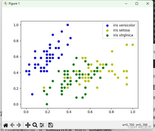
plt.scatter(iris_first[:, 0], iris_first[:, 1], c='b')
plt.scatter(iris_second[:, 0], iris_second[:, 1], c='y')
plt.scatter(iris_third[:, 0], iris_third[:, 1], c='g')
plt.legend(['iris versicolor', 'iris setosa', 'iris vlrglnica'])
plt.show()

结果如图所示：
在这里插入图片描述

4.5 实践：基于前馈神经网络完成鸢尾花分类

继续使用NNDL 实验四线性分类的鸢尾花分类任务，上面给出了iris数据集的介绍。将Softmax分类器替换为前馈神经网络。

损失函数：交叉熵损失；
优化器：随机梯度下降法；
评价指标：准确率。

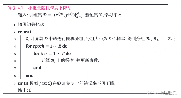
4.5.1 小批量梯度下降法

批量梯度下降法： 在梯度下降法中，目标函数是整个训练集上的风险函数，这种方式称为批量梯度下降法（Batch Gradient Descent，BGD）。批量梯度下降法在每次迭代时需要计算每个样本上损失函数的梯度并求和。当训练集中的样本数量 $N$ 很大时，空间复杂度比较高，每次迭代的计算开销也很大。

小批量梯度下降法： 为了减少每次迭代的计算复杂度，我们可以在每次迭代时只采集一小部分样本，计算在这组样本上损失函数的梯度并更新参数，这种优化方式称为小批量梯度下降法（Mini-Batch Gradient Descent，Mini-Batch GD）。

第 $\mathbb{t}$ 次迭代时，随机选取一个包含 $\mathbb{K}$ 个样本的子集 $\mathbb{Bt}$ ，计算这个子集上每个样本损失函数的梯度并进行平均，然后再进行参数更新。
$θ_{t+1}←θ_t−α\frac{1}{K}∑_{(x,y)∈S_t}\frac{∂L(y,f(x;θ))}{∂θ}$
其中 $K$ 为批量大小(Batch Size)。 $K$ 通常不会设置很大，一般在 $1 \sim 100$ 之间。在实际应用中为了提高计算效率，通常设置为 $2$ 的幂 $2^n$ 。

在实际应用中，小批量随机梯度下降法有收敛快、计算开销小的优点，因此逐渐成为大规模的机器学习中的主要优化算法。此外，随机梯度下降相当于在批量梯度下降的梯度上引入了随机噪声。在非凸优化问题中，随机梯度下降更容易逃离局部最优点。
小批量随机梯度下降法的训练过程如下：
在这里插入图片描述

为了小批量梯度下降法，我们需要对数据进行随机分组。
目前，机器学习中通常做法是构建一个数据迭代器，每个迭代过程中从全部数据集中获取一批指定数量的数据。

4.5.1.1 数据分组

为了小批量梯度下降法，我们需要对数据进行随机分组。目前，机器学习中通常做法是构建一个数据迭代器，每个迭代过程中从全部数据集中获取一批指定数量的数据。

数据迭代器的实现原理如下图所示：
在这里插入图片描述

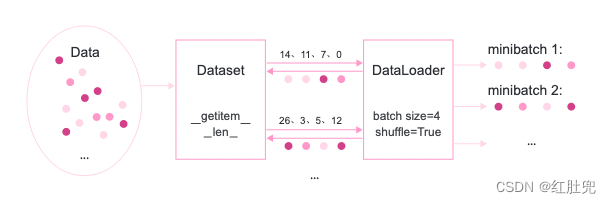
首先，将数据集封装为Dataset类，传入一组索引值，根据索引从数据集合中获取数据；
其次，构建DataLoader类，需要指定数据批量的大小和是否需要对数据进行乱序，通过该类即可批量获取数据。

在实践过程中，通常使用进行参数优化。在pytorch中，使用torch.utils.data.DataLoader加载minibatch的数据，torch.utils.data.DataLoader API可以生成一个迭代器，其中通过设置batch_size参数来指定minibatch的长度，通过设置shuffle参数为True，可以在生成minibatch的索引列表时将索引顺序打乱。

4.5.2 数据处理

构造IrisDataset类进行数据读取，继承自torch.utils.data.Dataset类。torch.utils.data.Dataset是用来封装 Dataset的方法和行为的抽象类，通过一个索引获取指定的样本，同时对该样本进行数据处理。当继承torch.utils.data.Dataset来定义数据读取类时，实现如下方法：

getitem：根据给定索引获取数据集中指定样本，并对样本进行数据处理；
len：返回数据集样本个数。

代码实现如下：

import torch
import numpy as np
import torch.utils.data
from nndl.load_data import load_data
 
 
class IrisDataset(torch.utils.data.Dataset):
    def __init__(self, mode='train', num_train=120, num_dev=15):
        super(IrisDataset, self).__init__()
        # 调用第三章中的数据读取函数，其中不需要将标签转成one-hot类型
        X, y = load_data(shuffle=True)
        if mode == 'train':
            self.X, self.y = X[:num_train], y[:num_train]
        elif mode == 'dev':
            self.X, self.y = X[num_train:num_train + num_dev], y[num_train:num_train + num_dev]
        else:
            self.X, self.y = X[num_train + num_dev:], y[num_train + num_dev:]
 
    def __getitem__(self, idx):
        return self.X[idx], self.y[idx]
 
    def __len__(self):
        return len(self.y)
 
 
torch.manual_seed(12)
train_dataset = IrisDataset(mode='train')
dev_dataset = IrisDataset(mode='dev')
test_dataset = IrisDataset(mode='test')
# 打印训练集长度
print("length of train set: ", len(train_dataset))

运行结果如下：
在这里插入图片描述

4.5.2.2 用DataLoader进行封装

# 批量大小
batch_size = 16
 
# 加载数据
train_loader = torch.utils.data.DataLoader(train_dataset, batch_size=batch_size, shuffle=True)
dev_loader = torch.utils.data.DataLoader(dev_dataset, batch_size=batch_size)
test_loader = torch.utils.data.DataLoader(test_dataset, batch_size=batch_size)

4.5.3 模型构建

构建一个简单的前馈神经网络进行鸢尾花分类实验。其中输入层神经元个数为4，输出层神经元个数为3，隐含层神经元个数为6。代码实现如下：

import torch.nn as nn
from torch.nn.init import constant_, normal_, uniform_
 
 
# 定义前馈神经网络
class Model_MLP_L2_V3(nn.Module):
    def __init__(self, input_size, output_size, hidden_size):
        super(Model_MLP_L2_V3, self).__init__()
        # 构建第一个全连接层
        self.fc1 = nn.Linear(input_size, hidden_size)
        normal_(self.fc1.weight, mean=0.0, std=0.01)
        constant_(self.fc1.bias, val=1.0)
        # 构建第二全连接层
        self.fc2 = nn.Linear(hidden_size, output_size)
        normal_(self.fc2.weight, mean=0.0, std=0.01)
        constant_(self.fc2.bias, val=1.0)
        # 定义网络使用的激活函数
        self.act = nn.Sigmoid()
 
    def forward(self, inputs):
        outputs = self.fc1(inputs)
        outputs = self.act(outputs)
        outputs = self.fc2(outputs)
        return outputs
 
 
fnn_model = Model_MLP_L2_V3(input_size=4, output_size=3, hidden_size=6)

4.5.4 完善Runner类

基于RunnerV2类进行完善实现了RunnerV3类。其中训练过程使用自动梯度计算，使用DataLoader加载批量数据，使用随机梯度下降法进行参数优化；模型保存时，使用state_dict方法获取模型参数；模型加载时，使用set_state_dict方法加载模型参数.

由于这里使用随机梯度下降法对参数优化，所以数据以批次的形式输入到模型中进行训练，那么评价指标计算也是分别在每个批次进行的，要想获得每个epoch整体的评价结果，需要对历史评价结果进行累积。这里定义Accuracy类实现该功能。

import torch
 
 
class Accuracy():
    def __init__(self, is_logist=True):
        """
        输入：
           - is_logist: outputs是logist还是激活后的值
        """
 
        # 用于统计正确的样本个数
        self.num_correct = 0
        # 用于统计样本的总数
        self.num_count = 0
 
        self.is_logist = is_logist
 
    def update(self, outputs, labels):
        """
        输入：
           - outputs: 预测值, shape=[N,class_num]
           - labels: 标签值, shape=[N,1]
        """
 
        # 判断是二分类任务还是多分类任务，shape[1]=1时为二分类任务，shape[1]>1时为多分类任务
        if outputs.shape[1] == 1: # 二分类
            outputs = torch.squeeze(outputs, dim=-1)
            if self.is_logist:
                # logist判断是否大于0
                preds = torch.tensor((outputs >= 0), dtype=torch.float32)
            else:
                # 如果不是logist，判断每个概率值是否大于0.5，当大于0.5时，类别为1，否则类别为0
                preds = torch.tensor((outputs >= 0.5), dtype=torch.float32)
        else:
            # 多分类时，使用'paddle.argmax'计算最大元素索引作为类别
            preds = torch.argmax(outputs, dim=1)
            preds = torch.tensor(preds, dtype=torch.int64)
 
        # 获取本批数据中预测正确的样本个数
        labels = torch.squeeze(labels, dim=-1)
        batch_correct = torch.sum(torch.tensor(preds == labels, dtype=torch.float32)).numpy()
        batch_count = len(labels)
 
        # 更新num_correct 和 num_count
        self.num_correct += batch_correct
        self.num_count += batch_count
 
    def accumulate(self):
        # 使用累计的数据，计算总的指标
        if self.num_count == 0:
            return 0
        return self.num_correct / self.num_count
 
    def reset(self):
        # 重置正确的数目和总数
        self.num_correct = 0
        self.num_count = 0
 
    def name(self):
        return "Accuracy"

RunnerV3类的代码实现如下：

class RunnerV3(object):
    def __init__(self, model, optimizer, loss_fn, metric, **kwargs):
        self.model = model
        self.optimizer = optimizer
        self.loss_fn = loss_fn
        self.metric = metric  # 只用于计算评价指标
 
        # 记录训练过程中的评价指标变化情况
        self.dev_scores = []
 
        # 记录训练过程中的损失函数变化情况
        self.train_epoch_losses = []  # 一个epoch记录一次loss
        self.train_step_losses = []  # 一个step记录一次loss
        self.dev_losses = []
 
        # 记录全局最优指标
        self.best_score = 0
 
    def train(self, train_loader, dev_loader=None, **kwargs):
        # 将模型切换为训练模式
        self.model.train()
 
        # 传入训练轮数，如果没有传入值则默认为0
        num_epochs = kwargs.get("num_epochs", 0)
        # 传入log打印频率，如果没有传入值则默认为100
        log_steps = kwargs.get("log_steps", 100)
        # 评价频率
        eval_steps = kwargs.get("eval_steps", 0)
 
        # 传入模型保存路径，如果没有传入值则默认为"best_model.pdparams"
        save_path = kwargs.get("save_path", "best_model.pdparams")
 
        custom_print_log = kwargs.get("custom_print_log", None)
 
        # 训练总的步数
        num_training_steps = num_epochs * len(train_loader)
 
        if eval_steps:
            if self.metric is None:
                raise RuntimeError('Error: Metric can not be None!')
            if dev_loader is None:
                raise RuntimeError('Error: dev_loader can not be None!')
 
        # 运行的step数目
        global_step = 0
 
        # 进行num_epochs轮训练
        for epoch in range(num_epochs):
            # 用于统计训练集的损失
            total_loss = 0
            for step, data in enumerate(train_loader):
                X, y = data
                # 获取模型预测
                logits = self.model(X)
                y = torch.tensor(y, dtype=torch.int64)
                loss = self.loss_fn(logits, y)  # 默认求mean
                total_loss += loss
 
                # 训练过程中，每个step的loss进行保存
                self.train_step_losses.append((global_step, loss.item()))
 
                if log_steps and global_step % log_steps == 0:
                    print(
                        f"[Train] epoch: {epoch}/{num_epochs}, step: {global_step}/{num_training_steps}, loss: {loss.item():.5f}")
 
                # 梯度反向传播，计算每个参数的梯度值
                loss.backward()
 
                if custom_print_log:
                    custom_print_log(self)
 
                # 小批量梯度下降进行参数更新
                self.optimizer.step()
                # 梯度归零
                self.optimizer.zero_grad()
 
                # 判断是否需要评价
                if eval_steps > 0 and global_step > 0 and \
                        (global_step % eval_steps == 0 or global_step == (num_training_steps - 1)):
 
                    dev_score, dev_loss = self.evaluate(dev_loader, global_step=global_step)
                    print(f"[Evaluate]  dev score: {dev_score:.5f}, dev loss: {dev_loss:.5f}")
 
                    # 将模型切换为训练模式
                    self.model.train()
 
                    # 如果当前指标为最优指标，保存该模型
                    if dev_score > self.best_score:
                        self.save_model(save_path)
                        print(
                            f"[Evaluate] best accuracy performence has been updated: {self.best_score:.5f} --> {dev_score:.5f}")
                        self.best_score = dev_score
 
                global_step += 1
 
            # 当前epoch 训练loss累计值
            trn_loss = (total_loss / len(train_loader)).item()
            # epoch粒度的训练loss保存
            self.train_epoch_losses.append(trn_loss)
 
        print("[Train] Training done!")
 
    # 模型评估阶段，使用'paddle.no_grad()'控制不计算和存储梯度
    @torch.no_grad()
    def evaluate(self, dev_loader, **kwargs):
        assert self.metric is not None
 
        # 将模型设置为评估模式
        self.model.eval()
 
        global_step = kwargs.get("global_step", -1)
 
        # 用于统计训练集的损失
        total_loss = 0
 
        # 重置评价
        self.metric.reset()
 
        # 遍历验证集每个批次
        for batch_id, data in enumerate(dev_loader):
            X, y = data
 
            # 计算模型输出
            logits = self.model(X)
            y = torch.tensor(y, dtype=torch.int64)
 
            # 计算损失函数
            loss = self.loss_fn(logits, y).item()
            # 累积损失
            total_loss += loss
 
            # 累积评价
            self.metric.update(logits, y)
 
        dev_loss = (total_loss / len(dev_loader))
        dev_score = self.metric.accumulate()
 
        # 记录验证集loss
        if global_step != -1:
            self.dev_losses.append((global_step, dev_loss))
            self.dev_scores.append(dev_score)
 
        return dev_score, dev_loss
 
    # 模型评估阶段，使用'paddle.no_grad()'控制不计算和存储梯度
    @torch.no_grad()
    def predict(self, x, **kwargs):
        # 将模型设置为评估模式
        self.model.eval()
        # 运行模型前向计算，得到预测值
        logits = self.model(x)
        return logits
 
    def save_model(self, save_path):
        torch.save(self.model.state_dict(), save_path)
 
    def load_model(self, model_path):
        model_state_dict = torch.load(model_path)
        self.model.set_state_dict(model_state_dict)

4.5.5 模型训练

实例化RunnerV3类，并传入训练配置，代码实现如下：

import torch.optim as opt
import torch.nn.functional as F
 
lr = 0.2
# 定义网络
model = fnn_model
# 定义优化器
optimizer = opt.SGD(lr=lr, params=model.parameters())
# 定义损失函数。softmax+交叉熵
loss_fn = F.cross_entropy
# 定义评价指标
metric = Accuracy(is_logist=True)
runner = RunnerV3(model, optimizer, loss_fn, metric)

使用训练集和验证集进行模型训练，共训练150个epoch。在实验中，保存准确率最高的模型作为最佳模型。代码实现如下：

# 启动训练
log_steps = 100
eval_steps = 50
runner.train(train_loader, dev_loader, num_epochs=150, log_steps=log_steps, eval_steps=eval_steps, save_path="best_model.pdparams")

运行结果：

[Train] epoch: 0/150, step: 0/1200, loss: 1.09898
[Evaluate]  dev score: 0.33333, dev loss: 1.09582
[Evaluate] best accuracy performence has been updated: 0.00000 --> 0.33333
[Train] epoch: 12/150, step: 100/1200, loss: 1.13891
[Evaluate]  dev score: 0.46667, dev loss: 1.10749
[Evaluate] best accuracy performence has been updated: 0.33333 --> 0.46667
[Evaluate]  dev score: 0.20000, dev loss: 1.10089
[Train] epoch: 25/150, step: 200/1200, loss: 1.10158
[Evaluate]  dev score: 0.20000, dev loss: 1.12477
[Evaluate]  dev score: 0.46667, dev loss: 1.09090
[Train] epoch: 37/150, step: 300/1200, loss: 1.09982
[Evaluate]  dev score: 0.46667, dev loss: 1.07537
[Evaluate]  dev score: 0.53333, dev loss: 1.04453
[Evaluate] best accuracy performence has been updated: 0.46667 --> 0.53333
[Train] epoch: 50/150, step: 400/1200, loss: 1.01054
[Evaluate]  dev score: 1.00000, dev loss: 1.00635
[Evaluate] best accuracy performence has been updated: 0.53333 --> 1.00000
[Evaluate]  dev score: 0.86667, dev loss: 0.86850
[Train] epoch: 62/150, step: 500/1200, loss: 0.63702
[Evaluate]  dev score: 0.80000, dev loss: 0.66986
[Evaluate]  dev score: 0.86667, dev loss: 0.57089
[Train] epoch: 75/150, step: 600/1200, loss: 0.56490
[Evaluate]  dev score: 0.93333, dev loss: 0.52392
[Evaluate]  dev score: 0.86667, dev loss: 0.45410
[Train] epoch: 87/150, step: 700/1200, loss: 0.41929
[Evaluate]  dev score: 0.86667, dev loss: 0.46156
[Evaluate]  dev score: 0.93333, dev loss: 0.41593
[Train] epoch: 100/150, step: 800/1200, loss: 0.41047
[Evaluate]  dev score: 0.93333, dev loss: 0.40600
[Evaluate]  dev score: 0.93333, dev loss: 0.37672
[Train] epoch: 112/150, step: 900/1200, loss: 0.42777
[Evaluate]  dev score: 0.93333, dev loss: 0.34534
[Evaluate]  dev score: 0.93333, dev loss: 0.33552
[Train] epoch: 125/150, step: 1000/1200, loss: 0.30734
[Evaluate]  dev score: 0.93333, dev loss: 0.31958
[Evaluate]  dev score: 0.93333, dev loss: 0.32091
[Train] epoch: 137/150, step: 1100/1200, loss: 0.28321
[Evaluate]  dev score: 0.93333, dev loss: 0.28383
[Evaluate]  dev score: 0.93333, dev loss: 0.27171
[Evaluate]  dev score: 0.93333, dev loss: 0.25447
[Train] Training done!

可视化观察训练集损失和训练集loss变化情况。

import matplotlib.pyplot as plt
 
 
# 绘制训练集和验证集的损失变化以及验证集上的准确率变化曲线
def plot_training_loss_acc(runner, fig_name,
                           fig_size=(16, 6),
                           sample_step=20,
                           loss_legend_loc="upper right",
                           acc_legend_loc="lower right",
                           train_color="#e4007f",
                           dev_color='#f19ec2',
                           fontsize='large',
                           train_linestyle="-",
                           dev_linestyle='--'):
    plt.figure(figsize=fig_size)
 
    plt.subplot(1, 2, 1)
    train_items = runner.train_step_losses[::sample_step]
    train_steps = [x[0] for x in train_items]
    train_losses = [x[1] for x in train_items]
 
    plt.plot(train_steps, train_losses, color=train_color, linestyle=train_linestyle, label="Train loss")
    if len(runner.dev_losses) > 0:
        dev_steps = [x[0] for x in runner.dev_losses]
        dev_losses = [x[1] for x in runner.dev_losses]
        plt.plot(dev_steps, dev_losses, color=dev_color, linestyle=dev_linestyle, label="Dev loss")
    # 绘制坐标轴和图例
    plt.ylabel("loss", fontsize=fontsize)
    plt.xlabel("step", fontsize=fontsize)
    plt.legend(loc=loss_legend_loc, fontsize='x-large')
 
    # 绘制评价准确率变化曲线
    if len(runner.dev_scores) > 0:
        plt.subplot(1, 2, 2)
        plt.plot(dev_steps, runner.dev_scores,
                 color=dev_color, linestyle=dev_linestyle, label="Dev accuracy")
 
        # 绘制坐标轴和图例
        plt.ylabel("score", fontsize=fontsize)
        plt.xlabel("step", fontsize=fontsize)
        plt.legend(loc=acc_legend_loc, fontsize='x-large')
 
    plt.savefig(fig_name)
    plt.show()
 
 
plot_training_loss_acc(runner, 'fw-loss.pdf')

运行结果如下：
在这里插入图片描述

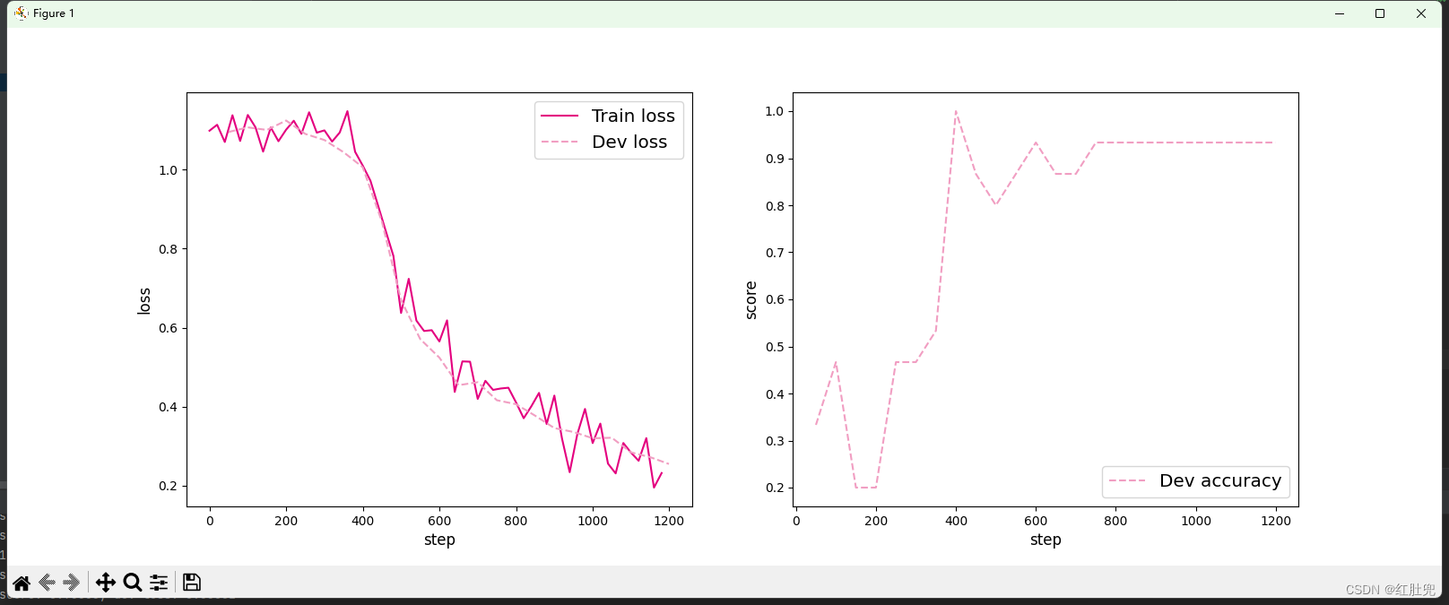
从输出结果可以看出准确率随着迭代次数增加逐渐上升，损失函数下降。

4.5.6 模型评价

使用测试数据对在训练过程中保存的最佳模型进行评价，观察模型在测试集上的准确率以及Loss情况。代码实现如下：

# 加载最优模型
runner.load_model('best_model.pdparams')
# 模型评价
score, loss = runner.evaluate(test_loader)
print("[Test] accuracy/loss: {:.4f}/{:.4f}".format(score, loss))

运行结果如下：
在这里插入图片描述

4.5.7 模型预测

同样地，也可以使用保存好的模型，对测试集中的某一个数据进行模型预测，观察模型效果。代码实现如下：

# 模型评价
score, loss = runner.evaluate(test_loader)
print("[Test] accuracy/loss: {:.4f}/{:.4f}".format(score, loss))
test_loader = iter(test_loader)
# 获取测试集中第一条数据
(X, label) = next(test_loader)
logits = runner.predict(X)
pred_class = torch.argmax(logits[0]).numpy()
label = label.numpy()[0]
 
# 输出真实类别与预测类别
print("The true category is {} and the predicted category is {}".format(label, pred_class))

运行结果如下：
在这里插入图片描述

思考题

对比Softmax分类和前馈神经网络分类。（必做）
（1）Softmax实现对鸢尾花进行分类结果：

import numpy as np
import matplotlib.pyplot as plt
from sklearn import datasets
from sklearn.linear_model import LogisticRegression
from matplotlib.colors import ListedColormap
 
iris = datasets.load_iris()  # 加载数据
list(iris.keys())  # 属性
X = iris["data"][:, (2, 3)]  # 花瓣长度, 花瓣宽度
y = iris["target"]
# 设置超参数multi_class为"multinomial"，指定一个支持Softmax回归的求解器，默认使用l2正则化，可以通过超参数C进行控制
softmax_reg = LogisticRegression(multi_class="multinomial", solver="lbfgs", C=500, random_state=42)
softmax_reg.fit(X, y)
softmax_reg.predict([[5, 2]])  # 输出：array([2])
softmax_reg.predict_proba([[5, 2]])
x0, x1 = np.meshgrid(np.linspace(0, 8, 500).reshape(-1, 1), np.linspace(0, 3.5, 200).reshape(-1, 1))
X_new = np.c_[x0.ravel(), x1.ravel()]
y_proba = softmax_reg.predict_proba(X_new)
y_predict = softmax_reg.predict(X_new)
zz1 = y_proba[:, 1].reshape(x0.shape)
zz = y_predict.reshape(x0.shape)
plt.figure(figsize=(10, 4))
plt.plot(X[y == 2, 0], X[y == 2, 1], "g^", label="Iris virginica")
plt.plot(X[y == 1, 0], X[y == 1, 1], "bs", label="Iris versicolor")
plt.plot(X[y == 0, 0], X[y == 0, 1], "yo", label="Iris setosa")
custom_cmap = ListedColormap(['#fafab0', '#9898ff', '#a0faa0'])
plt.contourf(x0, x1, zz, cmap=custom_cmap)
plt.xlabel("Petal length", fontsize=14)
plt.ylabel("Petal width", fontsize=14)
plt.legend(loc="center left", fontsize=14)
plt.axis([0, 7, 0, 3.5])
plt.show()

在这里插入图片描述

在这里插入图片描述

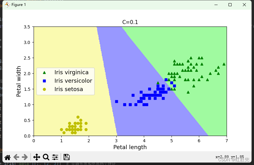
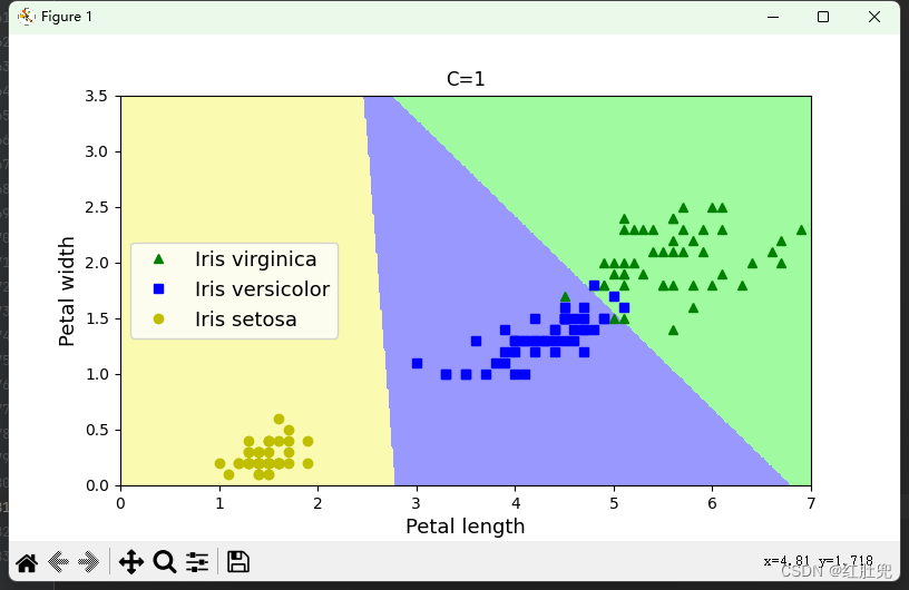
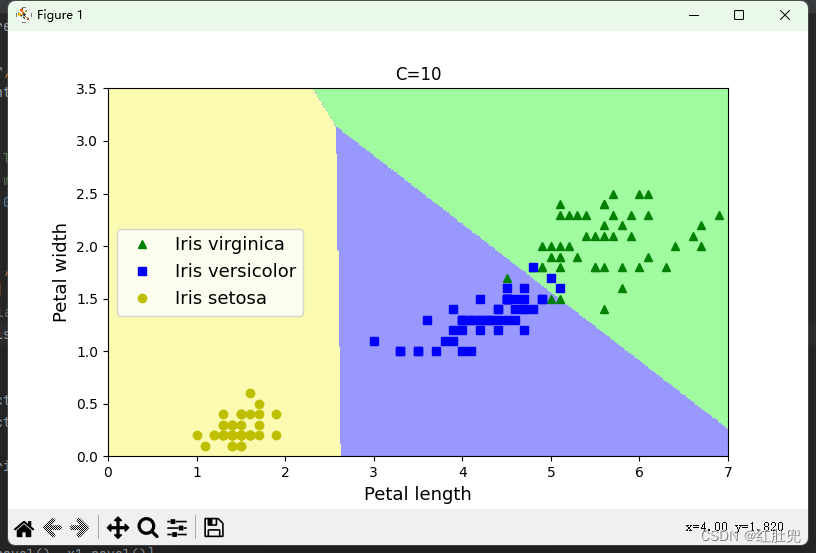
Softmax分类结果：

前馈神经网络分类结果：

从结果上来看，前馈神经网络分类的准确率要明显高于Softmax分类。

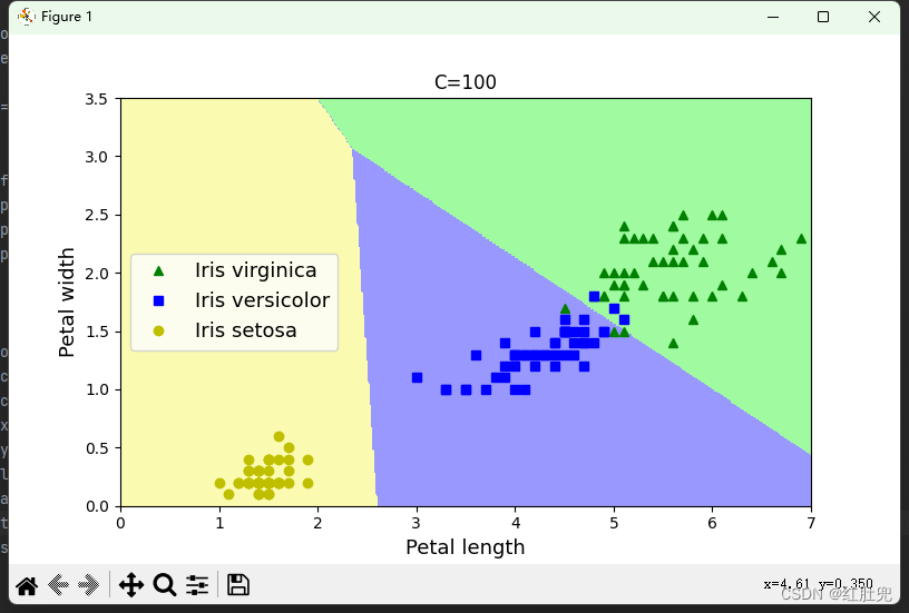
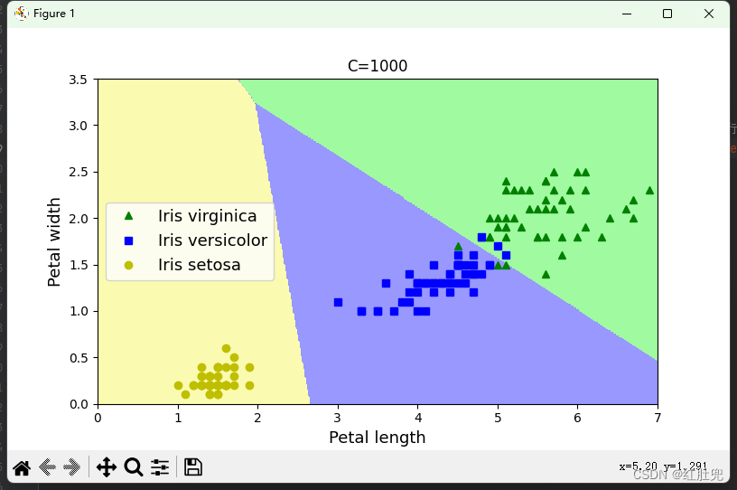
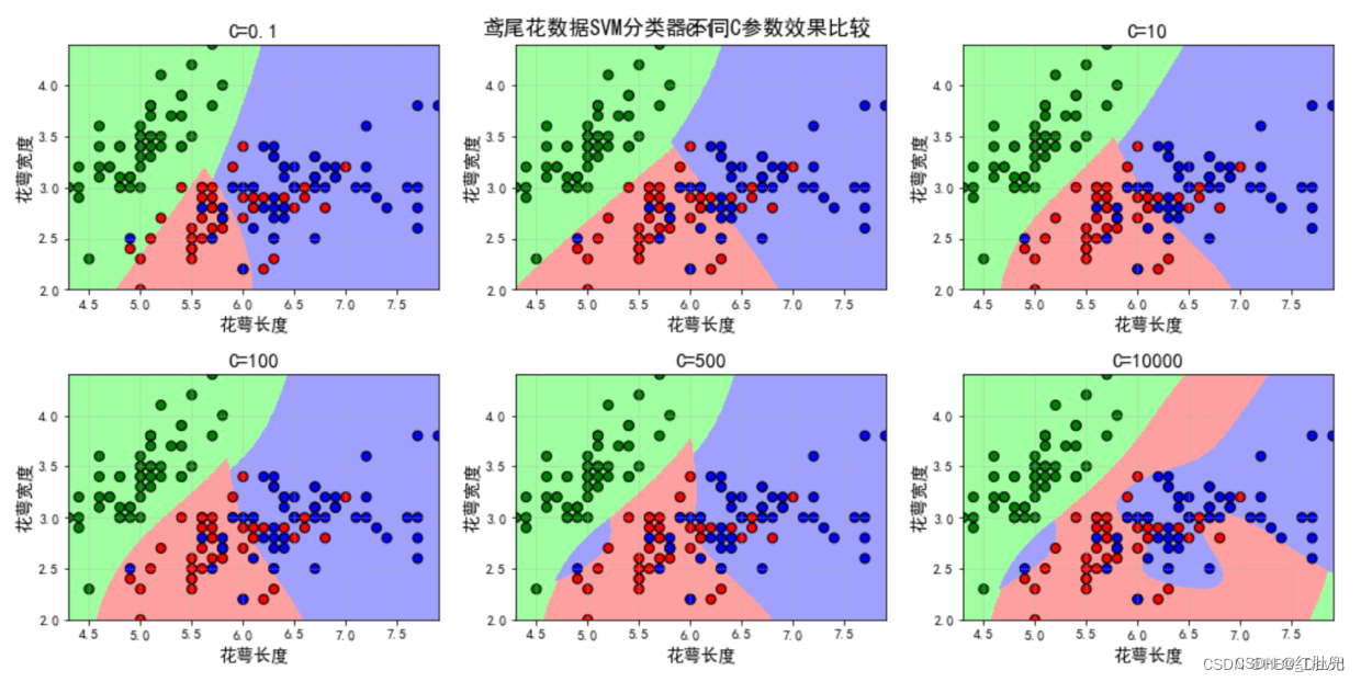
对比SVM与FNN分类效果，谈谈自己看法。
SVM（支持向量机）训练代码如下：

import math  # 数学
import random  # 随机
import numpy as np
import matplotlib.pyplot as plt
import matplotlib as mpl
mpl.rcParams['font.sans-serif'] = u'SimHei'
 
def zhichi_w(zhichi, xy, a):  # 计算更新 w
    w = [0, 0]
    if len(zhichi) == 0:  # 初始化的0
        return w
    for i in zhichi:
        w[0] += a[i] * xy[0][i] * xy[2][i]  # 更新w
        w[1] += a[i] * xy[1][i] * xy[2][i]
    return w
 
 
def zhichi_b(zhichi, xy, a):  # 计算更新 b
    b = 0
    if len(zhichi) == 0:  # 初始化的0
        return 0
    for s in zhichi:  # 对任意的支持向量有 ysf(xs)=1 所有支持向量求解平均值
        sum = 0
        for i in zhichi:
            sum += a[i] * xy[2][i] * (xy[0][i] * xy[0][s] + xy[1][i] * xy[1][s])
        b += 1 / xy[2][s] - sum
    return b / len(zhichi)
 
 
def SMO(xy, m):
    a = [0.0] * len(xy[0])  # 拉格朗日乘子
    zhichi = set()  # 支持向量下标
    loop = 1  # 循环标记（符合KKT）
    w = [0, 0]  # 初始化 w
    b = 0  # 初始化 b
    while loop:
        loop += 1
        if loop == 150:
            print("达到早停标准")
            print("循环了：", loop, "次")
            loop = 0
            break
        # 初始化=========================================
        fx = []  # 储存所有的fx
        yfx = []  # 储存所有yfx-1的值
        Ek = []  # Ek,记录fx-y用于启发式搜索
        E_ = -1  # 贮存最大偏差，减少计算
        a1 = 0  # SMO  a1
        a2 = 0  # SMO  a2
        # 初始化结束======================================
        # 寻找a1,a2======================================
        for i in range(len(xy[0])):  # 计算所有的 fx yfx-1 Ek
            fx.append(w[0] * xy[0][i] + w[1] * xy[1][i] + b)  # 计算 fx=wx+b
            yfx.append(xy[2][i] * fx[i] - 1)  # 计算 yfx-1
            Ek.append(fx[i] - xy[2][i])  # 计算 fx-y
            if i in zhichi:  # 之前看过的不看了，防止重复找某个a
                continue
            if yfx[i] <= yfx[a1]:
                a1 = i  # 得到偏离最大位置的下标(数值最小的)
        if yfx[a1] >= 0:  # 最小的也满足KKT
            print("循环了：", loop, "次")
            loop = 0  # 循环标记（符合KKT）置零(没有用到)
            break
        for i in range(len(xy[0])):  # 遍历找间隔最大的a2
            if i == a1:  # 如果是a1，跳过
                continue
            Ei = abs(Ek[i] - Ek[a1])  # |Eki-Eka1|
            if Ei < E_:  # 找偏差
                E_ = Ei  # 储存偏差的值
                a2 = i  # 储存偏差的下标
        # 寻找a1,a2结束===================================
        zhichi.add(a1)  # a1录入支持向量
        zhichi.add(a2)  # a2录入支持向量
        # 分析约束条件=====================================
        # c=a1*y1+a2*y2
        c = a[a1] * xy[2][a1] + a[a2] * xy[2][a2]  # 求出c
        # n=K11+k22-2*k12
        if m == "xianxinghe":  # 线性核
            n = xy[0][a1] ** 2 + xy[1][a1] ** 2 + xy[0][a2] ** 2 + xy[1][a2] ** 2 - 2 * (
                    xy[0][a1] * xy[0][a2] + xy[1][a1] * xy[1][a2])
        elif m == "duoxiangshihe":  # 多项式核(这里是二次)
            n = (xy[0][a1] ** 2 + xy[1][a1] ** 2) ** 2 + (xy[0][a2] ** 2 + xy[1][a2] ** 2) ** 2 - 2 * (
                    xy[0][a1] * xy[0][a2] + xy[1][a1] * xy[1][a2]) ** 2
        else:  # 高斯核  取 2σ^2 = 1
            n = 2 * math.exp(-1) - 2 * math.exp(-((xy[0][a1] - xy[0][a2]) ** 2 + (xy[1][a1] - xy[1][a2]) ** 2))
        # 确定a1的可行域=====================================
        if xy[2][a1] == xy[2][a2]:
            L = max(0.0, a[a1] + a[a2] - 0.5)  # 下界
            H = min(0.5, a[a1] + a[a2])  # 上界
        else:
            L = max(0.0, a[a1] - a[a2])  # 下界
            H = min(0.5, 0.5 + a[a1] - a[a2])  # 上界
        if n > 0:
            a1_New = a[a1] - xy[2][a1] * (Ek[a1] - Ek[a2]) / n  # a1_New = a1_old-y1(e1-e2)/n
            # print("x1=",xy[0][a1],"y1=",xy[1][a1],"z1=",xy[2][a1],"x2=",xy[0][a2],"y2=",xy[1][a2],"z2=",xy[2][a2],"a1_New=",a1_New)
            # 越界裁剪============================================================
            if a1_New >= H:
                a1_New = H
            elif a1_New <= L:
                a1_New = L
        else:
            a1_New = min(H, L)
        # 参数更新=======================================
        a[a2] = a[a2] + xy[2][a1] * xy[2][a2] * (a[a1] - a1_New)  # a2更新
        a[a1] = a1_New  # a1更新
        w = zhichi_w(zhichi, xy, a)  # 更新w
        b = zhichi_b(zhichi, xy, a)  # 更新b
        # print("W=", w, "b=", b, "zhichi=", zhichi, "a1=", a[a1], "a2=", a[a2])
    # 标记支持向量======================================
    for i in zhichi:
        if a[i] == 0:  # 选了，但值仍为0
            loop = loop + 1
            e = 'silver'
        else:
            if xy[2][i] == 1:
                e = 'b'
            else:
                e = 'r'
        plt.scatter(x1[0][i], x1[1][i], c='none', s=100, linewidths=1, edgecolor=e)
    print("支持向量数为：", len(zhichi), "\na为零支持向量：", loop)
    print("有用向量数：", len(zhichi) - loop)
    # 返回数据 w b =======================================
    return [w, b]
 
 
def panduan(xyz, w_b1, w_b2):
    c = 0
    for i in range(len(xyz[0])):
        if (xyz[0][i] * w_b1[0][0] + xyz[1][i] * w_b1[0][1] + w_b1[1]) * xyz[2][i][0] < 0:
            c = c + 1
            continue
        if (xyz[0][i] * w_b2[0][0] + xyz[1][i] * w_b2[0][1] + w_b2[1]) * xyz[2][i][1] < 0:
            c = c + 1
            continue
    return (1 - c / len(xyz[0])) * 100
 
 
def huitu(x1, x2, wb1, wb2, name):
    x = [x1[0][:], x1[1][:], x1[2][:]]
    for i in range(len(x[2])):  # 对训练集‘上色’
        if x[2][i] == [1, 1]:
            x[2][i] = 'r'  # 训练集  1  1 红色
        elif x[2][i] == [-1, 1]:
            x[2][i] = 'g'  # 训练集 -1  1 绿色
        else:
            x[2][i] = 'b'  # 训练集 -1 -1 蓝色
    plt.scatter(x[0], x[1], c=x[2], alpha=0.8)  # 绘点训练集
    x = [x2[0][:], x2[1][:], x2[2][:]]
    for i in range(len(x[2])):  # 对测试集‘上色’
        if x[2][i] == [1, 1]:
            x[2][i] = 'orange'  # 训练集  1   1 橙色
        elif x[2][i] == [-1, 1]:
            x[2][i] = 'y'  # 训练集 -1   1 黄色
        else:
            x[2][i] = 'm'  # 训练集 -1  -1 紫色
    plt.scatter(x[0], x[1], c=x[2], alpha=0.8)  # 绘点测试集
    plt.xlabel('x')  # x轴标签
    plt.ylabel('y')  # y轴标签
    plt.title(name)  # 标题
    xl = np.arange(min(x[0]), max(x[0]), 0.1)  # 绘制分类线一
    yl = (-wb1[0][0] * xl - wb1[1]) / wb1[0][1]
    plt.plot(xl, yl, 'r')
    xl = np.arange(min(x[0]), max(x[0]), 0.1)  # 绘制分类线二
    yl = (-wb2[0][0] * xl - wb2[1]) / wb2[0][1]
    plt.plot(xl, yl, 'b')
 
 
# 主函数=======================================================
f = open('Iris.txt', 'r')  # 读文件
x = [[], [], [], [], []]  # 花朵属性，(0,1,2,3),花朵种类
while 1:
    yihang = f.readline()  # 读一行
    if len(yihang) <= 1:  # 读到末尾结束
        break
    fenkai = yihang.split('\t')  # 按\t分开
    for i in range(4):  # 分开的四个值
        x[i].append(eval(fenkai[i]))  # 化为数字加到x中
    if (eval(fenkai[4]) == 1):  # 将标签化为向量形式
        x[4].append([1, 1])
    else:
        if (eval(fenkai[4]) == 2):
            x[4].append([-1, 1])
        else:
            x[4].append([-1, -1])
 
print('数据集=======================================================')
print(len(x[0]))  # 数据大小
# 选择数据===================================================
shuxing1 = eval(input("选取第一个属性："))
if shuxing1 < 0 or shuxing1 > 4:
    print("无效选项，默认选择第1项")
    shuxing1 = 1
shuxing2 = eval(input("选取第一个属性："))
if shuxing2 < 0 or shuxing2 > 4 or shuxing1 == shuxing2:
    print("无效选项，默认选择第2项")
    shuxing2 = 2
# 生成数据集==================================================
lt = list(range(150))  # 得到一个顺序序列
random.shuffle(lt)  # 打乱序列
x1 = [[], [], []]  # 初始化x1
x2 = [[], [], []]  # 初始化x2
for i in lt[0:100]:  # 截取部分做训练集
    x1[0].append(x[shuxing1][i])  # 加上数据集x属性
    x1[1].append(x[shuxing2][i])  # 加上数据集y属性
    x1[2].append(x[4][i])  # 加上数据集c标签
for i in lt[100:150]:  # 截取部分做测试集
    x2[0].append(x[shuxing1][i])  # 加上数据集x属性
    x2[1].append(x[shuxing2][i])  # 加上数据集y属性
    x2[2].append(x[4][i])  # 加上数据集c标签
print('\n\n开始训练==============================================')
print('\n线性核==============================================')
# 计算 w b============================================
plt.figure(1)  # 第一张画布
x = [x1[0][:], x1[1][:], []]  # 第一次分类
for i in x1[2]:
    x[2].append(i[0])  # 加上数据集标签
wb1 = SMO(x, "SVM")
x = [x1[0][:], x1[1][:], []]  # 第二次分类
for i in x1[2]:
    x[2].append(i[1])  # 加上数据集标签
wb2 = SMO(x, "SVM")
print("w1为：", wb1[0], " b1为：", wb1[1])
print("w2为：", wb2[0], " b2为：", wb2[1])
# 计算正确率===========================================
print("训练集上的正确率为：", panduan(x1, wb1, wb2), "%")
print("测试集上的正确率为：", panduan(x2, wb1, wb2), "%")
# 绘图 ===============================================
# 圈着的是曾经选中的值，灰色的是选中但更新为0
huitu(x1, x2, wb1, wb2, "SVM")
print('\n多项式核============================================')
# 计算 w b============================================
plt.figure(2)  # 第二张画布
x = [x1[0][:], x1[1][:], []]  # 第一次分类
for i in x1[2]:
    x[2].append(i[0])  # 加上数据集标签
wb1 = SMO(x, "SVM")
x = [x1[0][:], x1[1][:], []]  # 第二次分类
for i in x1[2]:
    x[2].append(i[1])  # 加上数据集标签
wb2 = SMO(x, "SVM")
print("w1为：", wb1[0], " b1为：", wb1[1])
print("w2为：", wb2[0], " b2为：", wb2[1])
# 计算正确率===========================================
print("训练集上的正确率为：", panduan(x1, wb1, wb2), "%")
print("测试集上的正确率为：", panduan(x2, wb1, wb2), "%")
# 绘图 ===============================================
# 圈着的是曾经选中的值，灰色的是选中但更新为0
huitu(x1, x2, wb1, wb2, "SVM")
print('\n高斯核==============================================')
# 计算 w b============================================
plt.figure(3)  # 第三张画布
x = [x1[0][:], x1[1][:], []]  # 第一次分类
for i in x1[2]:
    x[2].append(i[0])  # 加上数据集标签
wb1 = SMO(x, "SVM")
x = [x1[0][:], x1[1][:], []]  # 第二次分类
for i in x1[2]:
    x[2].append(i[1])  # 加上数据集标签
wb2 = SMO(x, "SVM")
print("w1为：", wb1[0], " b1为：", wb1[1])
print("w2为：", wb2[0], " b2为：", wb2[1])
# 计算正确率===========================================
print("训练集上的正确率为：", panduan(x1, wb1, wb2), "%")
print("测试集上的正确率为：", panduan(x2, wb1, wb2), "%")
# 绘图 ===============================================
# 圈着的是曾经选中的值，灰色的是选中但更新为0
huitu(x1, x2, wb1, wb2, "SVM")
# 显示所有图
plt.show()  # 显示

运行结果：

数据集=======================================================
150
选取第一个属性：1
选取第一个属性：2


开始训练==============================================
循环了： 3 次
支持向量数为： 2 
a为零支持向量： 0
有用向量数： 2
循环了： 55 次
支持向量数为： 54 
a为零支持向量： 44
有用向量数： 10
w1为： [0.6000000000000001, -1.2]  b1为： 1.38
w2为： [-0.34999999999999987, -1.0]  b2为： 5.924444444444445
训练集上的正确率为： 92.0 %
测试集上的正确率为： 94.0 %

FNN分类效果图可参考：
在这里插入图片描述

SVM的优缺点
1、SVM算法对大规模训练样本难以实施
SVM的空间消耗主要是存储训练样本和核矩阵，由于SVM是借助二次规划来求解支持向量，而求解二次规划将涉及m阶矩阵的计算（m为样本的个数），当m数目很大时该矩阵的存储和计算将耗费大量的机器内存和运算时间。针对以上问题的主要改进有有J.Platt的SMO算法、T.Joachims的SVM、C.J.C.Burges等的PCGC、张学工的CSVM以及O.L.Mangasarian等的SOR算法。如果数据量很大，SVM的训练时间就会比较长，如垃圾邮件的分类检测，没有使用SVM分类器，而是使用了简单的naive
bayes分类器，或者是使用逻辑回归模型分类。

2、用SVM解决多分类问题存在困难
经典的支持向量机算法只给出了二类分类的算法，而在数据挖掘的实际应用中，一般要解决多类的分类问题。可以通过多个二类支持向量机的组合来解决。主要有一对多组合模式、一对一组合模式和SVM决策树；再就是通过构造多个分类器的组合来解决。主要原理是克服SVM固有的缺点，结合其他算法的优势，解决多类问题的分类精度。如：与粗集理论结合，形成一种优势互补的多类问题的组合分类器。

3、对缺失数据敏感，对参数和核函数的选择敏感
支持向量机性能的优劣主要取决于核函数的选取,所以对于一个实际问题而言,如何根据实际的数据模型选择合适的核函数从而构造SVM算法。目前比较成熟的核函数及其参数的选择都是人为的,根据经验来选取的,带有一定的随意性.在不同的问题领域,核函数应当具有不同的形式和参数,所以在选取时候应该将领域知识引入进来,但是目前还没有好的方法来解决核函数的选取问题。

参考文献

对比SVM与CNN对文本分类的效果_CodingPark编程公园
 HBU-NNDL 实验五前馈神经网络（3）鸢尾花分类
在这里插入图片描述

总结

这次作业通过使用前馈神经网络完成鸢尾花分类任务，在此深化理解了前馈神经网络的基本概念，此外还复习了SVM的知识点。神经网络最大的优势在数据量很大时才能体现出来。不得不承认好多函数还是不太会用，不太理解使用方法，做思考题之前还好，几个思考题都不太会做。好多还是照猫画虎，照葫芦画瓢。以后还要多下功夫。

红肚兜

关注

3
点赞
踩
5

收藏

觉得还不错? 一键收藏
打赏
0
评论
NNDL 实验五前馈神经网络（3）鸢尾花分类

鸢尾花数据集也就是iris数据集，是一个非常经典的数据集，各路大神一定并不陌生。这次实验我们就以此为实验来源，对鸢尾花进行分类。为防止有的同学不知道这个数据集，下面给出这个数据集以及可视化深入了解一下。可视化的代码如下：结果如图所示：继续使用NNDL 实验四线性分类的鸢尾花分类任务，上面给出了iris数据集的介绍。将Softmax分类器替换为前馈神经网络。批量梯度下降法：在梯度下降法中，目标函数是整个训练集上的风险函数，这种方式称为批量梯度下降法（Batch Gradient Des
复制链接

扫一扫