语音信号处理之时域特征、频谱特征、MFCC特征、语谱图特征、谱熵图特征的提取与可视化

        一、准备工作

        首先你需要有一段音频.....，不用太长，我是准备了一个八秒的无损音频，可以用专门的录音软件（例如：Audacity），或者可以下载一些音频然后转为无损（当然有损也可以提取特征），频率最好在16000Hz及以上。其次是你需要在你的python环境中安装以下库，我以pycharm社区版为例。

import numpy as np
import matplotlib.pyplot as plt
from python_speech_features import mfcc
from python_speech_features import delta
from sklearn.preprocessing import StandardScaler
import librosa.display
import pyworld

        二、提取

        2.1 读取音频文件

这里我是准备了两个方法，两个方法有一点点不同，稍微注意一下也是可以的

        2.1.1 使用librosa库提取（我是用的这个）。这个的特点是会将你的音频转为单声道，但是不会改变你音频的原有频率，如果想要改为16000Hz或者其他频率，可以加一个参数sr输入频率修改。

y, sr = librosa.load("audio.wav")

        2.1.2 使用pyworld库提取。这个的特点就是他会将你的音频转为单声道，但是会默认将你的频率改为16000Hz。

y, sr = pyworld.load("audio.wav")

  如果没有下载这个库可以从python解释器里面搜索下载也可以在终端内输入命令下载：

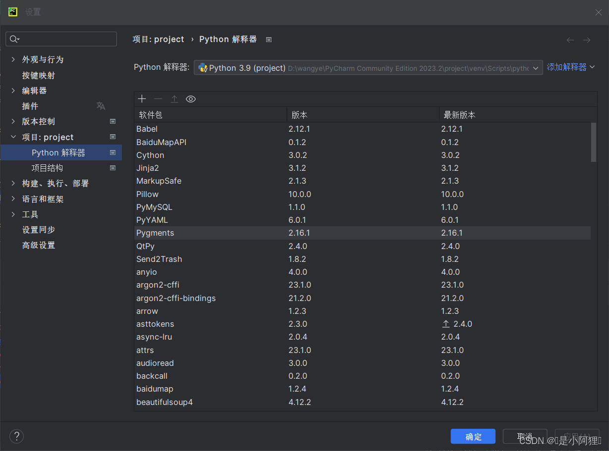
        2.1.2.1 解释器里面下载（我经常用这种方法，偶尔有些库某种原因这样子下载不了我才用终端）。在如下图片中点 + 号搜索下载。

        2.1.2.2 终端命令下载。如下图，输入命令下载。

        三、计算及其可视化

         3.1 时域特征

# 可视化时域特征
time = np.arange(len(y)) / sr
plt.figure(figsize=(14, 5))
plt.subplot(2, 1, 1)
plt.plot(time, y)
plt.xlabel('Time (s)')
plt.ylabel('Amplitude')
plt.title('Time-domain features')
plt.tight_layout()
plt.show()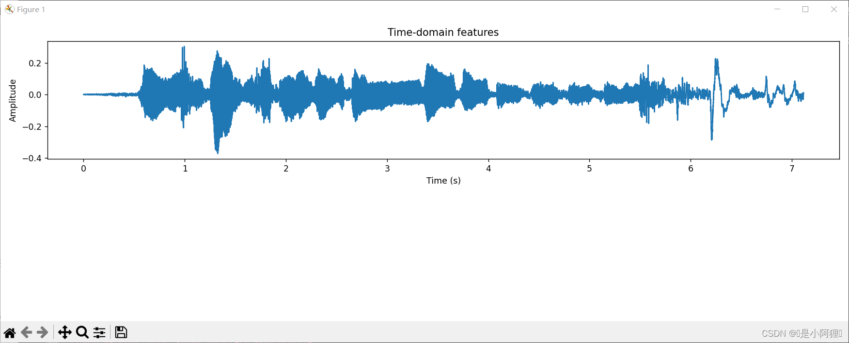

        3.2 频谱特征

# 可视化频域特征
D = librosa.stft(y)
D_db = librosa.amplitude_to_db(np.abs(D), ref=np.max)
plt.subplot(2, 1, 2)
librosa.display.specshow(D_db, sr=sr, x_axis='time', y_axis='log')
plt.colorbar(format='%+2.0f dB')
plt.title('Frequency-domain features')
plt.tight_layout()
plt.show()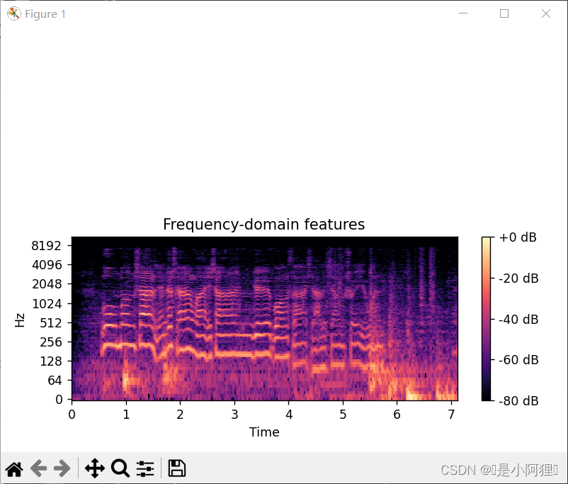

        3.3 MFCC特征

        3.3.1 转化。需要先将得到的音频数据和采样率转化为MFCC特征，在进行二阶时频变化。这个变化可以反映出音频信号的动态特性。

# 将音频转化为MFCC特征
mfcc_features = mfcc(y, sr)
# 对MFCC特征进行delta处理
delta_features = delta(mfcc_features, 2)

        3.3.2 归一化处理。因为特征间的单位（尺度）可能不同，在进行距离有关的计算时，单位的不同会导致计算结果的不同。

# 归一化处理
scaler = StandardScaler()
normalized_features = scaler.fit_transform(delta_features)

        3.3.3 可视化。

# 可视化MFCC特征
plt.figure(figsize=(10, 5))
plt.imshow(normalized_features.T, origin='lower', aspect='auto', cmap='jet')
plt.title('MFCC features')
plt.xlabel('Frame index')
plt.ylabel('MFCC coefficient index')
plt.tight_layout()
plt.show()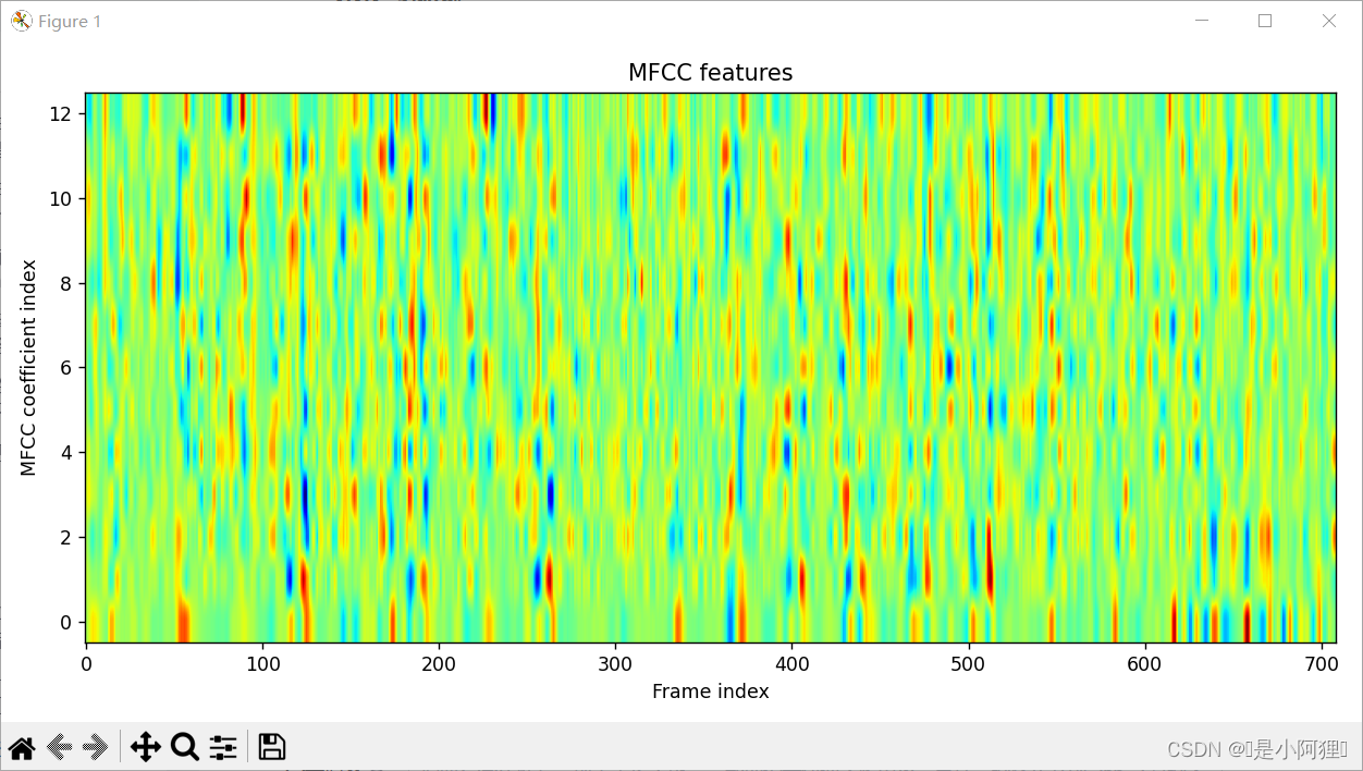

         3.4 语谱图特征

# 计算语谱图
S = librosa.feature.melspectrogram(y=y, sr=sr)

# 转换为分贝单位
S_db = librosa.power_to_db(S, ref=np.max)

# 可视化语谱图
plt.figure(figsize=(10, 5))
librosa.display.specshow(S_db, sr=sr, x_axis='time', y_axis='mel')
plt.colorbar(format='%+2.0f dB')
plt.title('Mel Spectrogram')
plt.tight_layout()
plt.show()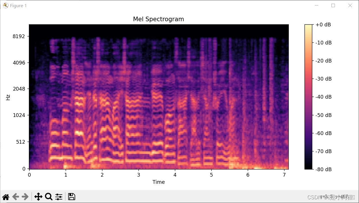

 

         3.5 谱熵图特征

# 计算短时傅里叶变换（STFT）
D = librosa.stft(y)
# 将STFT的幅度谱转换为概率分布
P = librosa.amplitude_to_db(np.abs(D), ref=np.max)
P = P / np.sum(P, axis=0)
# 计算谱熵
spectral_entropy = -np.sum(P * np.log2(P), axis=0)

plt.plot(spectral_entropy)
plt.xlabel('Frame index')
plt.ylabel('Spectral Entropy')
plt.title('Spectral Entropy Feature')
plt.show()

         四、结语

        上述特征是语音信号处理中很常见的一些特征，如果对你有帮助的话，我将会很开心。