


逻辑回归是一种广泛使用的统计学习方法,主要用于处理二分类问题。它基于线性回归模型,通过Sigmoid函数将输出映射到[0, 1]范围内,表示实例属于正类别的概率。尽管逻辑回归适用于二分类任务,但在多分类问题中常使用Softmax函数,它将多个类别的概率输出为和为1的正值,允许模型进行多类别预测。PyTorch是一个灵活且强大的深度学习框架,以其动态计算图和易用性受到广泛欢迎,适用于研究和生产环境中的各种机器学习任务。
一、sigmoid激活函数
1.1、输入散点
import numpy as np

class1_points = np.array([[1.9, 1.2],
                          [1.5, 2.1],
                          [1.9, 0.5],
                          [1.5, 0.9],
                          [0.9, 1.2],
                          [1.1, 1.7],
                          [1.4, 1.1]])

class2_points = np.array([[3.2, 3.2],
                          [3.7, 2.9],
                          [3.2, 2.6],
                          [1.7, 3.3],
                          [3.4, 2.6],
                          [4.1, 2.3],
                          [3.0, 2.9]])
x_train = np.concatenate((class1_points, class2_points))
y_train = np.concatenate((np.zeros(len(class1_points)), np.ones(len(class2_points))))
1.2、转换为Tensor张量
import torch
inputs=torch.tensor(x_train,dtype=torch.float32)
labels=torch.tensor(y_train,dtype=torch.float32).unsqueeze(1)
1.3、定义模型
import torch
import torch.nn as nn
torch.manual_seed(42)
class LogisticRegreModel(nn.Module):
    def __init__(self,inputsizes):
        super().__init__()
        self.linear=nn.Linear(inputsizes,1)
    def forward(self,x):
        return torch.sigmoid(self.linear(x))
model=LogisticRegreModel(x_train.shape[1])
1.4、定义损失函数和优化器
from torch.optim import SGD
cri=torch.nn.BCELoss()
optimizer=SGD(model.parameters(),lr=0.05)
1.5、开始迭代
for i in range(1,1001):
    output=model(inputs)
    loss=cri(output,labels)

    optimizer.zero_grad()
    loss.backward()
    optimizer.step()

    if i%100==0 or i==1:
        print(i,loss.item())
1.6、可视化
from matplotlib import pyplot as plt
fig,(ax1,ax2)=plt.subplots(1,2)
epoch_list=[]
loss_list=[]

for i in range(1,1001):
    inputs=torch.tensor(x_train,dtype=torch.float32)
    labels=torch.tensor(y_train,dtype=torch.float32).unsqueeze(1)

    output=model(inputs)
    loss=cri(output,labels)

    optimizer.zero_grad()
    loss.backward()
    optimizer.step()

    if i%100==0 or i==1:
        print(i,loss.item())
        w1,w2=model.linear.weight.data.flatten()
        b=model.linear.bias.data[0]

        slope=-w1/w2
        intercept=-b/w2
        x_min,x_max=0,5
        x=np.array([x_min,x_max])
        y=slope*x+intercept

        ax1.clear()
        ax1.scatter(class1_points[:,0],class1_points[:,1])
        ax1.scatter(class2_points[:,0],class2_points[:,1])
        ax1.plot(x,y)

        ax2.clear()
        epoch_list.append(i)
        loss_list.append(loss.item())
        ax2.plot(epoch_list,loss_list)
plt.show()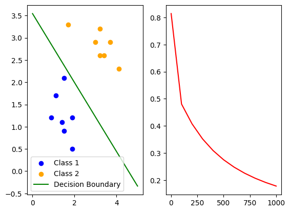
1.7、完整代码
import numpy as np  # 导入 NumPy 库以进行数组和数学运算
from matplotlib import pyplot as plt  # 导入 Matplotlib 库以绘制图形
import torch  # 导入 PyTorch 库
import torch.nn as nn  # 导入 PyTorch 的神经网络模块
from torch.optim import SGD  # 导入随机梯度下降优化器

# 定义类1的数据点
class1_points = np.array([[1.9, 1.2],
                          [1.5, 2.1],
                          [1.9, 0.5],
                          [1.5, 0.9],
                          [0.9, 1.2],
                          [1.1, 1.7],
                          [1.4, 1.1]])

# 定义类2的数据点
class2_points = np.array([[3.2, 3.2],
                          [3.7, 2.9],
                          [3.2, 2.6],
                          [1.7, 3.3],
                          [3.4, 2.6],
                          [4.1, 2.3],
                          [3.0, 2.9]])

# 合并类1和类2的数据点,作为训练特征
x_train = np.concatenate((class1_points, class2_points))
# 合并类1和类2的标签,类1为 0,类2为 1
y_train = np.concatenate((np.zeros(len(class1_points)), np.ones(len(class2_points))))

# 将训练特征和标签转换为 PyTorch 张量
inputs = torch.tensor(x_train, dtype=torch.float32)
labels = torch.tensor(y_train, dtype=torch.float32).unsqueeze(1)

# 设置随机种子以便复现结果
torch.manual_seed(42)

# 定义逻辑回归模型类
class LogisticRegreModel(nn.Module):
    def __init__(self, input_sizes):
        super().__init__()  # 继承父类的初始化方法
        self.linear = nn.Linear(input_sizes, 1)  # 定义线性层,输入大小为 input_sizes,输出为 1

    def forward(self, x):
        return torch.sigmoid(self.linear(x))  # 前向传播,应用 Sigmoid 函数

# 实例化逻辑回归模型,输入特征的维度为 x_train 的列数
model = LogisticRegreModel(x_train.shape[1])

# 定义二元交叉熵损失函数
cri = torch.nn.BCELoss()
# 使用随机梯度下降算法作为优化器
optimizer = SGD(model.parameters(), lr=0.05)

# 创建子图用于展示
fig, (ax1, ax2) = plt.subplots(1, 2)
epoch_list = []  # 存储每次训练的epoch数
loss_list = []   # 存储每次训练的损失值

# 训练模型,进行 1000 次迭代
for i in range(1, 1001):
    inputs = torch.tensor(x_train, dtype=torch.float32)  # 再次定义输入张量
    labels = torch.tensor(y_train, dtype=torch.float32).unsqueeze(1)  # 再次定义标签张量

    output = model(inputs)  # 前向传播计算模型输出
    loss = cri(output, labels)  # 计算损失值

    optimizer.zero_grad()  # 清空之前的梯度
    loss.backward()  # 反向传播计算梯度
    optimizer.step()  # 更新参数

    # 每 100 次迭代打印损失并更新图形
    if i % 100 == 0 or i == 1:
        print(i, loss.item())  # 打印当前epoch和损失值

        # 获取当前模型参数
        w1, w2 = model.linear.weight.data.flatten()  # 权重参数
        b = model.linear.bias.data[0]  # 偏置参数

        # 计算决策边界的斜率和截距
        slope = -w1 / w2
        intercept = -b / w2
        x_min, x_max = 0, 5  # 决定x轴的范围
        x = np.array([x_min, x_max])  # 创建x值的数组
        y = slope * x + intercept  # 根据斜率和截
                # 根据斜率和截距计算决策边界的y值
        y = slope * x + intercept

        ax1.clear()  # 清空第一张子图
        # 绘制类1和类2的数据点
        ax1.scatter(class1_points[:, 0], class1_points[:, 1], color='blue', label='Class 1')
        ax1.scatter(class2_points[:, 0], class2_points[:, 1], color='orange', label='Class 2')
        # 绘制当前的决策边界
        ax1.plot(x, y, color='green', label='Decision Boundary')
        ax1.legend()  # 显示图例

        ax2.clear()  # 清空第二张子图
        epoch_list.append(i)  # 将当前epoch添加到列表
        loss_list.append(loss.item())  # 将当前损失值添加到列表
        ax2.plot(epoch_list, loss_list, color='red')  # 绘制损失变化曲线

# 显示绘制的图形
plt.show()
二、Softmax激活函数
2.1、输入散点
import numpy as np

class1_points = np.array([[1.9, 1.2],
                          [1.5, 2.1],
                          [1.9, 0.5],
                          [1.5, 0.9],
                          [0.9, 1.2],
                          [1.1, 1.7],
                          [1.4, 1.1]])

class2_points = np.array([[3.2, 3.2],
                          [3.7, 2.9],
                          [3.2, 2.6],
                          [1.7, 3.3],
                          [3.4, 2.6],
                          [4.1, 2.3],
                          [3.0, 2.9]])
x_train = np.concatenate((class1_points, class2_points))
y_train = np.concatenate((np.zeros(len(class1_points)), np.ones(len(class2_points))))
2.2、转换为Tensor张量
import torch
inputs=torch.tensor(x_train,dtype=torch.float32)
labels=torch.tensor(y_train,dtype=torch.long)
2.3、定义模型
class LogisticRegreModel(torch.nn.Module):
    def __init__(self):
        super(LogisticRegreModel, self).__init__()
        self.fc = torch.nn.Linear(2, 2)

    def forward(self, x):
        x = self.fc(x)
        # dim 指定了softmax在哪个维度上进行
        # dim = 1第二个维度上进行,列
        # example:x  (sample, num_classes)
        # torch.softmax(x, dim=1), pytorch在每个样本上的类别进行softmax,保证每个样本的所有类别的概率和为1。
        return torch.softmax(x, dim=1)

model = LogisticRegreModel()
2.4、定义损失函数和优化器
cri = torch.nn.CrossEntropyLoss()
optimizer = torch.optim.SGD(model.parameters(), lr=0.05)
2.5、开始迭代
for epoch in range(1, 1001):

    outputs = model(inputs)
    loss = cri(outputs, labels)

    optimizer.zero_grad()
    loss.backward()
    optimizer.step()

    if epoch % 50 == 0 or epoch == 1:
        print(f"epoch: {epoch}, loss: {loss}")
2.6、可视化
plt.figure(figsize=(12, 6))

xx, yy = np.meshgrid(np.arange(0, 6, 0.1), np.arange(0, 6, 0.1))
grid_points = np.c_[xx.ravel(), yy.ravel()]

epoches = 1000
for epoch in range(1, epoches + 1):

    outputs = model(inputs)
    loss = cri(outputs, labels)

    optimizer.zero_grad()
    loss.backward()
    optimizer.step()

    if epoch % 50 == 0 or epoch == 1:
        print(f"epoch: {epoch}, loss: {loss}")
        grid_tensor = torch.tensor(grid_points, dtype=torch.float32)
        Z = model(grid_tensor).detach().numpy()
        Z = Z[:, 1]
        Z = Z.reshape(xx.shape)

        plt.cla()
        plt.scatter(class1_points[:, 0], class1_points[:, 1])
        plt.scatter(class2_points[:, 0], class2_points[:, 1])
        plt.contour(xx, yy, Z, levels=[0.5])
        plt.pause(1)

plt.show()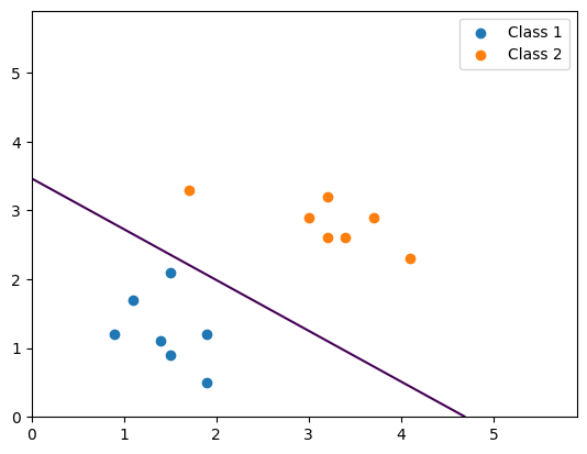
2.7、完整代码
import numpy as np  # 导入 NumPy 库进行数组和数学运算
import torch  # 导入 PyTorch 库
import matplotlib.pyplot as plt  # 导入 Matplotlib 用于绘图

# 定义类1的数据点
class1_points = np.array([[1.9, 1.2],
                          [1.5, 2.1],
                          [1.9, 0.5],
                          [1.5, 0.9],
                          [0.9, 1.2],
                          [1.1, 1.7],
                          [1.4, 1.1]])

# 定义类2的数据点
class2_points = np.array([[3.2, 3.2],
                          [3.7, 2.9],
                          [3.2, 2.6],
                          [1.7, 3.3],
                          [3.4, 2.6],
                          [4.1, 2.3],
                          [3.0, 2.9]])

# 合并类1和类2的数据点,作为训练特征
x_train = np.concatenate((class1_points, class2_points))
# 合并类1和类2的标签,类1为 0,类2为 1
y_train = np.concatenate((np.zeros(len(class1_points)), np.ones(len(class2_points))))

# 将训练特征和标签转换为 PyTorch 张量
inputs = torch.tensor(x_train, dtype=torch.float32)  # 输入特征
labels = torch.tensor(y_train, dtype=torch.long)  # 标签应为长整型

# 定义逻辑回归模型类
class LogisticRegreModel(torch.nn.Module):
    def __init__(self):
        super(LogisticRegreModel, self).__init__()  # 继承父类的初始化方法
        self.fc = torch.nn.Linear(2, 2)  # 定义线性层,输入大小为 2,输出类别数为 2

    def forward(self, x):
        x = self.fc(x)  # 进行前向传播,计算线性层输出
        # 使用 softmax 函数将输出转换为概率
        return torch.softmax(x, dim=1)  # dim=1 表示在列上进行 softmax 操作

# 实例化逻辑回归模型
model = LogisticRegreModel()

# 定义交叉熵损失函数,适用于多分类问题
cri = torch.nn.CrossEntropyLoss()
# 定义优化器为随机梯度下降
optimizer = torch.optim.SGD(model.parameters(), lr=0.05)

# 创建绘图窗口
plt.figure(figsize=(12, 6))

# 创建网格点用于绘制决策边界
xx, yy = np.meshgrid(np.arange(0, 6, 0.1), np.arange(0, 6, 0.1))  # 生成网格坐标
grid_points = np.c_[xx.ravel(), yy.ravel()]  # 将网格点展平为 (样本数, 特征数) 的形式

epoches = 1000  # 定义训练的轮数
for epoch in range(1, epoches + 1):
    outputs = model(inputs)  # 前向传播获得模型输出
    loss = cri(outputs, labels)  # 计算损失

    optimizer.zero_grad()  # 清空之前的梯度
    loss.backward()  # 反向传播计算梯度
    optimizer.step()  # 更新模型参数

    # 每 50 个 epoch 更新绘图
    if epoch % 50 == 0 or epoch == 1:
        print(f"epoch: {epoch}, loss: {loss.item()}")  # 打印当前 epoch 和损失值
        grid_tensor = torch.tensor(grid_points, dtype=torch.float32)  # 将网格点转换为张量
        Z = model(grid_tensor).detach().numpy()  # 前向传播获得每个网格点的输出
        Z = Z[:, 1]  # 取出第二类的概率,用于绘制决策边界
        Z = Z.reshape(xx.shape)  # 重塑为网格形状

        plt.cla()  # 清除当前图形
        plt.scatter(class1_points[:, 0], class1_points[:, 1], label='Class 1')  # 绘制类1数据点
        plt.scatter(class2_points[:, 0], class2_points[:, 1], label='Class 2')
        plt.contour(xx, yy, Z, levels=[0.5])
        plt.legend()
        plt.pause(1)

plt.show()


 被折叠的 条评论
为什么被折叠?
被折叠的 条评论
为什么被折叠?
 到【灌水乐园】发言


