matlab：绘图（2）

学习素材：MATLAB教程_台大郭彦甫（14课）原视频补档

MATLAB教學 - 06进阶绘图_哔哩哔哩_bilibili

（部分素材使用视频截图）

一、对数相关绘图

1.Logarithm plots 对数

semilogx(X,Y) 在 x 轴上使用以 10 为底的对数刻度、在 y 轴上使用线性刻度来绘制 x 和 y 坐标。

loglog(X,Y) 在 x 轴和 y 轴上应用以 10 为底的对数刻度来绘制 x 和 y 坐标。

>> x=logspace(-1,1,100);%生成10^--1到10^1的100个数据
>> subplot(2,2,1);
>> plot(x,y);
>> title('Plot');
>> subplot(2,2,2);
>> semilogx(x,y);
>> title('Semilogx');
>> subplot(2,2,3);
>> semilogy(x,y);
>> title('Semilogy');
>> subplot(2,2,4);
>> loglog(x,y);
>> title('loglog');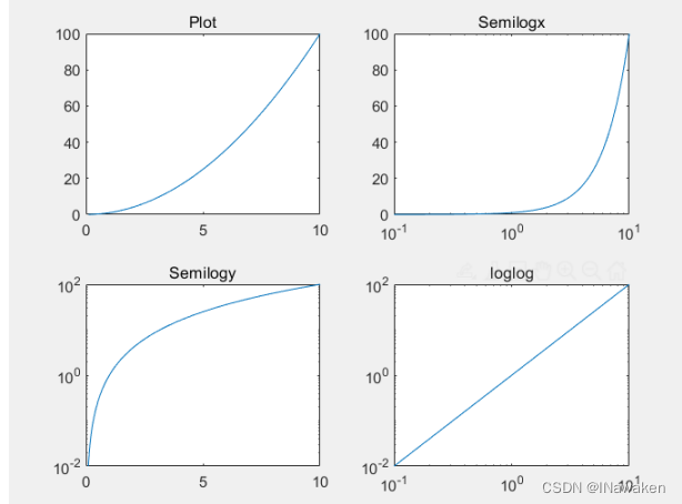

 

set(gca,'XGrid','on');

2. plotyy()

>> x=0:0.01:20;
>> y1=200*exp(-0.05*x).*sin(x);
>> y2=0.8*exp(-0.5*x).*sin(10*x);
>> [AX,H1,H2]=plotyy(x,y1,x,y2);
>> set(get(AX(1)),'Ylabel'),'String','Left Y-axis')
>> set(get(AX(1),'Ylabel'),'String','Left Y-axis')
>> set(get(AX(2),'Ylabel'),'String','Right Y-axis')
>> title('Labeling plotyy');
set(H1,'LineStyle','--');set(H2,'LineStyle',':');
%get查询图形对象属性
%AX:存储坐标轴信息
%H1,H2存储Line信息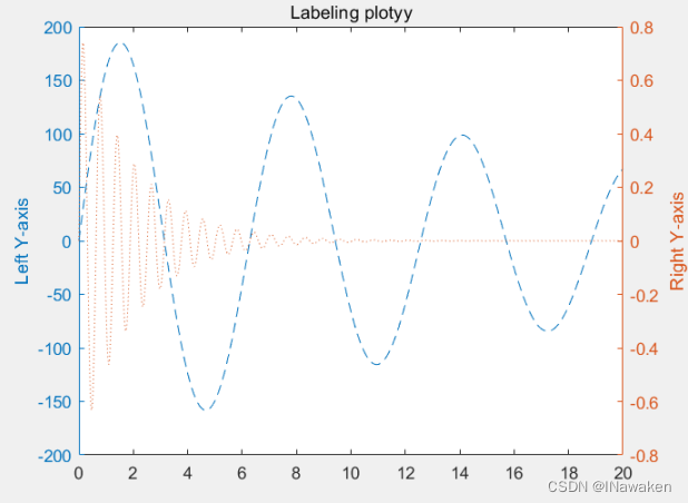

 二、Histogram and Pie Charts(直方图和饼图

1.hist

>> y=randn(1,1000);%randn正态分布随机数
subplot(2,1,1);
hist(y,10);
title('Bins=10');
>> subplot(2,1,2);
>> hist(y,50);
>> title('Bins=50');

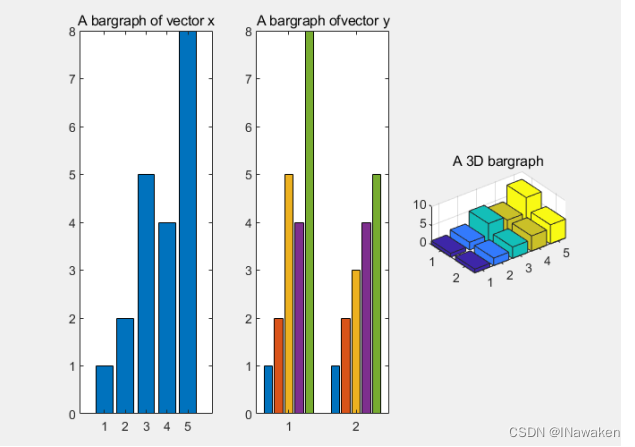
 2.Bar CHarts(柱形图)

>> x=[1 2 5 4 8];
>> y=[x;1:5];%矩阵
>>  subplot(1,3,1);bar(x);title('A bargraph of vector x');
>> subplot(1,3,2);bar(y);title('A bargraph ofvector y');
>> subplot(1,3,3);bar3(y);title('A 3D bargraph');
%bar3(z) 为 z 的元素创建一个三维条形图。每个条形对应于 z 中的一个元素。
%bar(y) 创建一个条形图，y 中的每个元素对应一个条形。
%如果 y 是 m×n 矩阵，则 bar 创建每组包含 n 个条形的 m 个组。

 

 3.Stack and Horizonral （成堆的，横向的）

'stacked' - 为 Y 中的每一行显示一个条形。条形高度是行中元素的总和。每个条形标记有多种颜色。不同颜色分别对应不同的元素，显示每行元素占总和的相对量。

Barh() 横向

>> x=[1 2 5 4 8];
>> y=[x;1:5];
>> subplot(1,2,1);
>> bar(y,'Stacked');
>> title('Stacked');
>> subplot(1,2,2);
>> barh(y);
>> title('Horizontal');

 

>> barh(y,'Stacked');

 4.Pie Charts （饼图

>> a=[10 5 20 30];
>> subplot(1,3,1);
>> pie(a);
>> subplot(1,3,2);
>> pie(a,[0,0,0,1]);
>> subplot(1,3,3);
>> pie3(a,[0,0,0,1]);

 

>> pie3(a,[0,1,2,3]);

 三、Polar Chart （极坐标图

Polar()

polar(theta,rho) 创建角 theta 对半径 rho 的极坐标图。theta 是从 x 轴到半径向量所夹的角（以弧度单位指定）；rho 是半径向量的长度（以数据空间单位指定）。

>> x=1:100;
>> theta=x/10;  r=log10(x);
>> subplot(1,4,1);  polar(theta,r);
>> theta = linspace(0,2*pi);  r=cos(4*theta);
>> subplot(1,4,2);  polar(theta,r);
>> theta=linspace(0,2*pi,6);r=ones(1,length(theta));%ones 构建全为1的1*length(theta)矩阵
>> subplot(1,4,3);polar(theta,r);
>> theta=linspace(0,2*pi);r=1-sin(theta);
>> subplot(1,4,4);polar(theta,r);

 六边形

>> theta=linspace(0,2*pi,7);r=ones(1,length(theta));
>> polar(theta,r);

四、其他二维绘图

 1.Stairs and Stem (阶梯图和离散序列数据)

作用：在固定时间取样

 

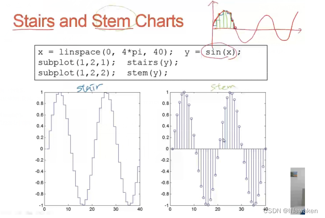
stairs(Y) 绘制 Y 中元素的阶梯图。

如果 Y 为向量，则 stairs 绘制一个线条。

如果 Y 为矩阵，则 stairs 为每个矩阵列绘制一个线条。

stem(Y) 将数据序列 Y 绘制为从沿 x 轴的基线延伸的针状图。各个数据值由终止每个针状图的圆指示。

如果 Y 是向量，x 轴的刻度范围是从 1 至 length(Y)。

如果 Y 是矩阵，则 stem 将根据相同的 x 值绘制行中的所有元素，并且 x 轴的刻度范围是从 1 至 Y 中的行数。

>> x=linspace(0,4*pi,40);y=sin(x);
>> subplot(1,2,1); stairs(y);
>> subplot(1,2,2); stem(y);

 例：

>> t=linspace(0,10);
>> y=sin((pi.*t.^2)./4);
>> stem(y);
>> hold on
>> plot(y);
>> hold off
>> yticks(-1:0.5:1);

2.Boxplot and Error Bar (用箱线图可视化汇总统计量和含误差条的线图

Boxplot

用箱线图可视化汇总统计量 - MATLAB boxplot - MathWorks 中国

Errorbar

含误差条的线图 - MATLAB errorbar - MathWorks 中国

>> load carsmall;
>> boxplot(MPG,Origin);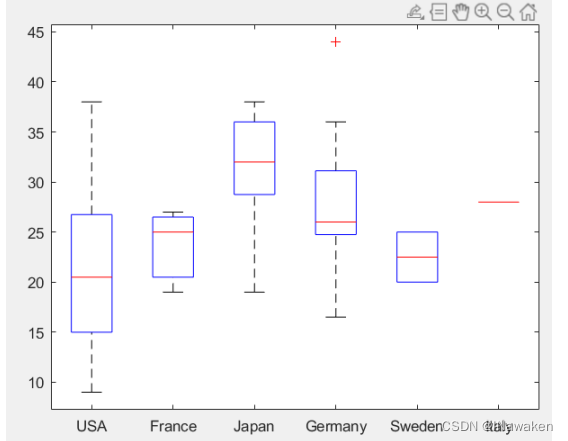

>> x=0:pi/10:pi; y=sin(x);
>> e=std(y)*ones(size(x)); %std:标准差
>> errorbar(x,y,e); %e为误差大小

 五、Fill()二维填充补片

t=(1:2:15)’*pi/8;推导过程

x=sin(t); y=cos(t);推导过程

 

 

>> t=(1:2:15)'*pi/8;
>> x=sin(t);
>> y=cos(t);
>> fill(x,y,'r');Z
>> axis square off;
>> text(0,0,'STOP','Color','w','FontSize',80,...
'FontWeight','bold','HorizontalAlignment','center');
%'FontWeight','bold' 字体加粗
%HorizontalAlignment 相对于点，水平对齐文本

 例、

 t=(1:1:4)'*pi/2;
x=sin(t);
y=cos(t);
fill(x,y,'y');
>> text(0,0,'WAIT','Color','k','FontSize',80,...
'FontWeight','bold','HorizontalAlignment','center');

 六、颜色设置

1.color space

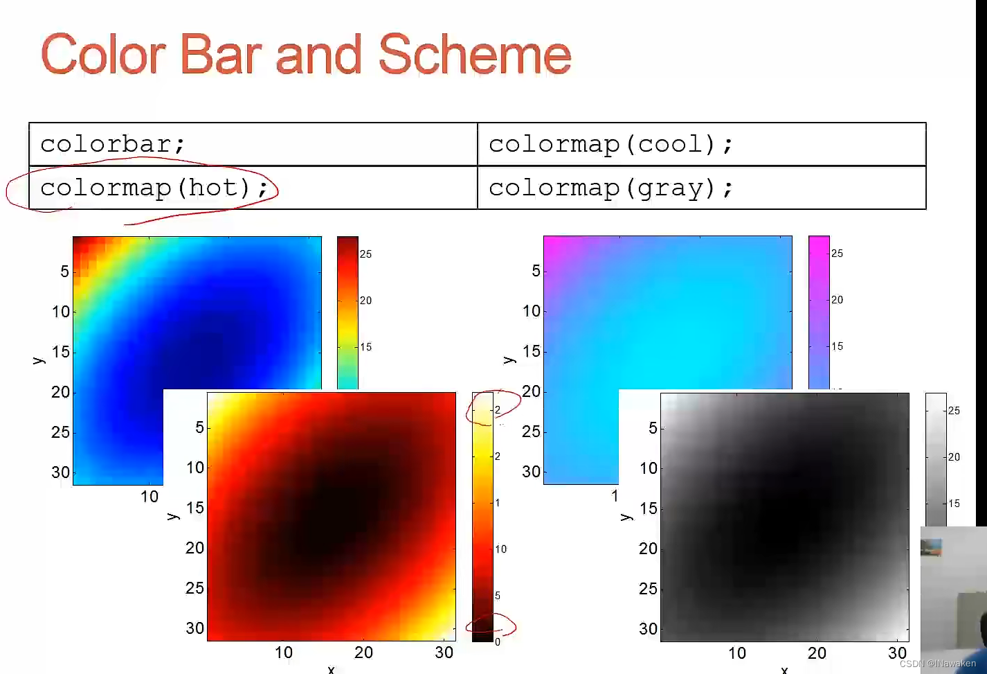
 2.Imagesc()使用缩放颜色显示图像

>> [x,y] =meshgrid(-3:.2:3,-3:.2:3);
>> z=x.^2+x.*y+y.^2;
>> surf(x,y,z);
>> box on;
>> set(gca,'FontSize',16);
>> zlabel('z');
>> xlim([-4,4]);
>> xlabel('X');
>> ylim([-4 4]);
>> ylabel('Y');
>> figure
>> imagesc(z);
>> axis square;
>> xlabel('x');
>> ylabel('y');

colorbar;

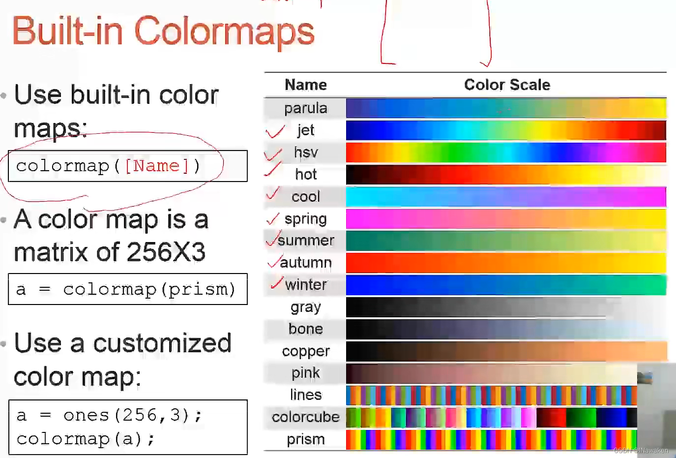
3.Colormap()

查看并设置当前颜色图 - MATLAB colormap - MathWorks 中国

七、3D plots

plot3()

>> x=0:0.1:3*pi;
>> z1=sin(x);
>> z2=sin(2*x);
>> z3=sin(3*x);
>> y1=zeros(size(x));
>> y3=ones(size(x));
>> y2=y3./2;
>> plot3(x,y1,z1,'r',x,y2,z2,'b',x,y3,z3,'g');
>> grid on
>> xlabel('x-axis');
>> ylabel('y-axis');
>> zlabel('z-axis');

>> t=0:pi/50:10*pi;
>> plot3(sin(t),cos(t),t);
>> grid on;
>> axis square;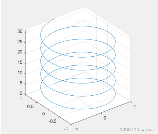

>> t=0:pi/50:10*pi;
>> plot3(sin(t),cos(t),t);
>> grid on;
>> axis square;
>> turns=40*pi;
>> t=linspace(0,turns,4000);
>> x=cos(t).*(turns-t)./turns;
>>  y=sin(t).*(turns-t)./turns;
>> z=t./turns;
>> plot3(x,y,z);
>> grid on;

八、3D surface

Meshgrid();

[X,Y] = meshgrid(x,y) 基于向量 x 和 y 中包含的坐标返回二维网格坐标。X 是一个矩阵，每一行是 x 的一个副本；Y 也是一个矩阵，每一列是 y 的一个副本。坐标 X 和 Y 表示的网格有 length(y) 个行和 length(x) 个列。

>> x=-3.5:0.2:3.5;
>> y=-3.5:0.2:3.5;
>> [x,y]=meshgrid(x,y);
>> z=x.*exp(-x.^2-y.^2);
>> subplot(1,2,1); mesh(x,y,z); %有实色边颜色，无面颜色
>> subplot(1,2,2); surf(x,y,z); %有实色边和实色面的三维曲面

九、Contour()

contour(Z) 创建一个包含矩阵 Z 的等值线的等高线图，其中 Z 包含 x-y 平面上的高度值。MATLAB® 会自动选择要显示的等高线。Z 的列和行索引分别是平面中的 x 和 y 坐标。

contour(X,Y,Z) 指定 Z 中各值的 x 和 y 坐标。

>> x=-3.5:0.2:3.5;
>> y=-3.5:0.2:3.5;
>> [X,Y]=meshgrid(x,y);
>> Z=X.*exp(-X.^2-Y.^2);
>> subplot(1,2,1);
>> mesh(X,Y,Z);
>> axis square;
>> subplot(1,2,2);
>> contour(X,Y,Z);%矩阵的等高线图
>> axis square;

 

>> x=-3.5:0.2:3.5;
y=-3.5:0.2:3.5;
>> [X,Y]=meshgrid(x,y);
>> Z=X.*exp(-X.^2-Y.^2);
>> subplot(1,3,1);
>> contour(Z,[-.45:.05:.45]);%指定高度处绘制等高线
>> axis square;
>> subplot(1,3,2);
>> [C,h]=contour(Z);
>> clabel(C,h);
>> axis square;
>> subplot(1,3,3);
>> contourf(Z); %f:fill();
>> axis square;

>> [C,h]=contourf(Z,[-.45:.05:.45]);
>> x=-3.5:0.2:3.5;
>>y=-3.5:0.2:3.5;
>>[X,Y]=meshgrid(x,y);
>>Z=X.*exp(-X.^2-Y.^2);
>> [C,h]=contourf(Z,[-.45:.05:.45]);
>> clabel(C,h);%为等高线图添加高程标签
>> axis square

十、Meshc() and surfc()

在mesh()和surf()的基础上绘制contour

>> x=-3.5:0.2:3.5;
>> y=-3.5:0.2:3.5;
>> [X,Y]=meshgrid(x,y);
>> Z=X.*exp(-X.^2-Y.^2);
>> subplot(1,2,1);
>> meshc(X,Y,Z);
>> subplot(1,2,2);
>> surfc(X,Y,Z);

 十六、view、ligt、patch

view()

相机视线 - MATLAB view - MathWorks 中国

light()

创建光源对象 - MATLAB light - MathWorks 中国

patch()

绘制一个或多个填充多边形区域 - MATLAB patch - MathWorks 中国

>> %绘制一个球
>> sphere(50);
>> shading flat;
>>  light('Position',[1 3 2]);
>> light('Position',[-3,-1,3]);
>> meterial shiny;
>> set(gcf,'Color',[1  1  1]);
>> view(-45,20);

 例、

>> load cape;
>> X=conv2(ones(9,9)/81,cumsum(cumsum(randn(100,100)),2));
>> surf(X,'EdgeColor','none','EdgeLighting','Phong',...
'FaceColor','interp');
>> colormap(map);
>> caxis([-10,300]);
>> grid off;
>> axis off;