有效投资边界的python实现

写作业吧

已于 2022-12-06 18:52:34 修改

阅读量1.9k

点赞数 2

文章标签： python 开发语言人工智能

于 2022-12-06 18:49:04 首次发布

本文链接：https://blog.csdn.net/weixin_67522489/article/details/128207865

版权

马科维茨有效投资投资边界的基本思想是通过对资产组合当中不同资产的配置情况进行调整，达到在既定风险水平下的收益最大化，或者既定收益水平下的风险最小化。

from datetime import date
import pandas_datareader.data as web
import matplotlib.pyplot as plt
import numpy as np 
import seaborn as sns
import warnings
warnings.filterwarnings("ignore")
%matplotlib inline

#获取股票数据
tickers = {
    'AAPL':'苹果',
    'AMZN':'亚马逊',
    'GOOGL':'谷歌',
    'BABA':'阿里巴巴'

}
data_source = 'stooq'#定义数据源的参数

start = date(2016,1,1)#起始时间

end = date(2017,12,31)#结束时间

stock_data = web.DataReader(list(tickers), data_source,start,end)["Close"]

stock_data.rename(columns=tickers,inplace=True)

stock_data=stock_data.iloc[::-1]
stock_data.head()

#画出收盘价走势图
sns.set_style("whitegrid")#横坐标有标线，纵坐标没有标线，背景白色
sns.set_style("darkgrid") #默认，横纵坐标都有标线，组成一个一个格子，背景稍微深色
sns.set_style("dark")#背景稍微深色，没有标线线
sns.set_style("white")#背景白色，没有标线线
sns.set_style("ticks")#xy轴都有非常短的小刻度
sns.despine(offset=30,left=True)#去掉上边和右边的轴线，offset=30表示距离轴线（x轴）的距离,left=True表示左边的轴保留


sns.set(font='SimHei',rc={'figure.figsize':(10,6)})# 图片大小和中文字体设置
# 图形展示

# name=input("股票名字")
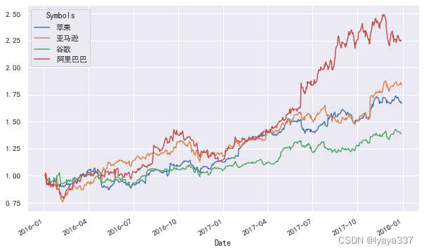
(stock_data/stock_data.iloc[0]).plot()

计算收益率和风险

收益率

$R_t=\frac{p_t-p_{t-1}}{p_t}=\frac{p_t}{P_{t-1}}-1$

对数收益率

$r=ln\frac{p_t}{p_{t-1}}$

年化收益率

$r\_annual=exp^{\sum^n_{i=1}\ r_i\times250}-1$

R=stock_data/stock_data.shift(1)-1
R.head()

log_r=np.log(stock_data/stock_data.shift(1))
log_r.head()

r_annual=np.exp(log_r.mean()*250)-1
r_annual

风险

std = np.sqrt(log_r.var() * 250)#假设协方差为0
std

投资组合的收益和风险

def gen_weights(n):
    w=np.random.rand(n)
    return w /sum(w)

n=len(list(tickers))
w=gen_weights(n)
list(zip(r_annual.index,w))

投资组合的收益

$\mu_p=\sum_{i=1}^nw_i\mu_i$

#投资组合收益
def port_ret(w):
    return np.sum(w*r_annual)
port_ret(w)

投资组合的风险

$\sigma^2=\sum^n_{i=1}\sum^n_{j=1}w_iw_jcov(r_i,r_j)$

#投资组合的风险
def port_std(w):
    return np.sqrt((w.dot(log_r.cov()*250).dot(w.T)))
port_std(w)

#若干投资组合的收益和风险

def gen_ports(times):
    for _ in range(times):#生成不同的组合
        w=gen_weights(n)#每次生成不同的权重
        yield (port_std(w),port_ret(w),w)#计算风险和期望收益 以及组合的权重情况

import pandas as pd 
df=pd.DataFrame(gen_ports(25000),columns=["std","ret","w"])
df.head()

引入夏普比率

$Sharpe\_Ratio=\frac{r_p-r_f}{\sigma_p}$

假设无风险利率为0.03，画出投资有效边界

df['sharpe'] = (df['ret'] - 0.015) / df['std']#定义夏普比率
fig, ax = plt.subplots()
df.plot.scatter('std', 'ret', c='sharpe',s=30, alpha=0.3, cmap='cool',marker='o', ax=ax)
plt.style.use('ggplot')
plt.rcParams['axes.unicode_minus'] = False# 显示负号

list(zip(r_annual.index, df.loc[df.sharpe.idxmax()].w))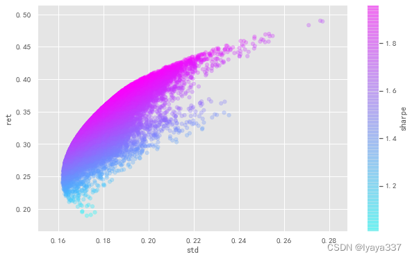

import scipy.optimize as opt
frontier=pd.DataFrame(columns=['std','ret'])

for std in np.linspace(0.16,0.25):
    res=opt.minimize(lambda x:-port_ret(x),
                x0=((1/n),)*n,
                method='SLSQP',
                bounds=((0,1),)*n,
                constraints=[
                   {"fun":lambda x:port_std(x)-std,"type":"eq"},
                   {"fun":lambda x:(np.sum(x)-1),"type":"eq"}
                ])
    if res.success:
        frontier=frontier.append({"std":std,"ret":-res.fun},ignore_index=True)
frontier.plot('std','ret',lw=3,c='blue',ax=ax)

fig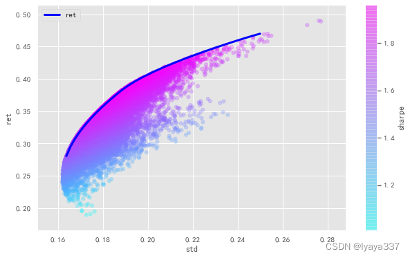

计算最优资产配置情况

res=opt.minimize(lambda x:-((port_ret(x)-0.03)/port_std(x)),
                x0=((1/n),)*n,
                method='SLSQP',
                bounds=((0,1),)*n,
                constraints={"fun":lambda x:(np.sum(x)-1), "type":"eq"})

res.x.round(3)

array([0.29 , 0.255, 0.   , 0.455])最优资产组合的配置为29%的苹果股票，25.5%的亚马逊股票，45.5%的阿里巴巴股票

ax.scatter(port_std(res.x),port_ret(res.x),marker="*",c="black",s=300)
fig

绘制资本市场线

ax.plot((0,.27),(.03,-res.fun*.27+.03))
fig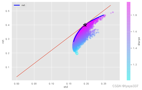

在上图的所示资本市场线上，星号左边表示将资本用于投资一部分无风险资产，和一部分风险资产组合，而在星号处代表将所有的资本都用于投资风险资产组合星号右边意味着借入无风险资产并投资于风险资产组合，可以在相同的风险水平下获得更高的收益。