集成学习基础

1. 使用鸢尾花数据分别训练集成模型：AdaBoost模型，Gradient Boosting模型

2. 对别两个集成模型的准确率以及报告

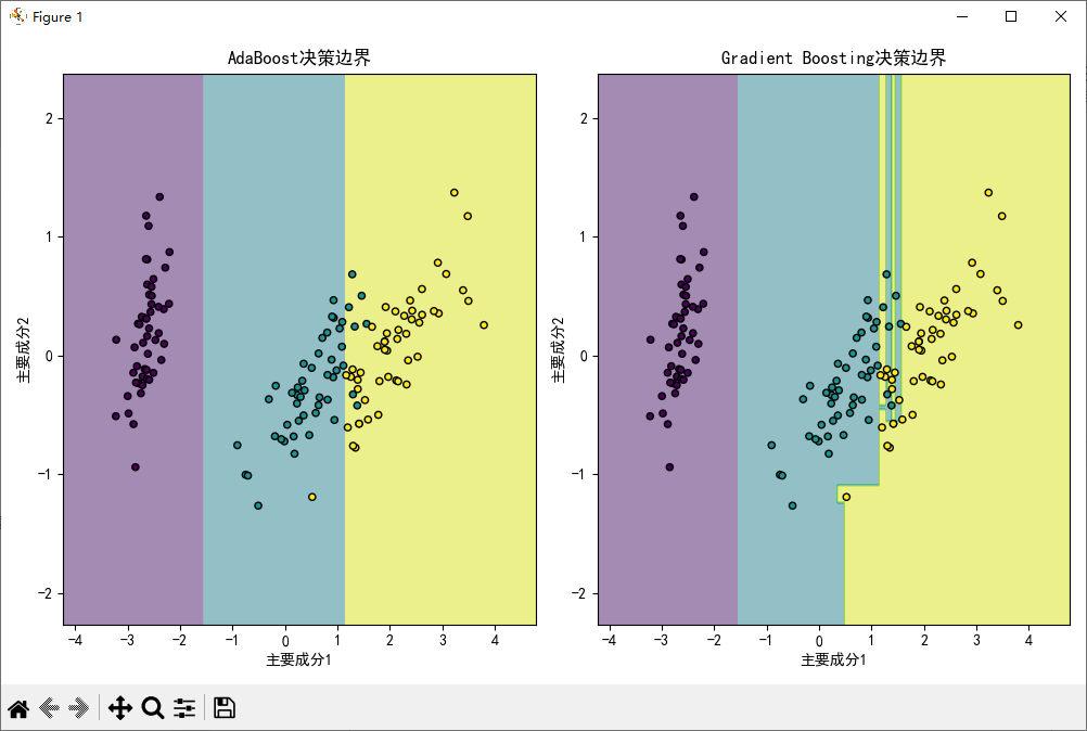
3. 两个模型的预测结果进行可视化 需要进行降维处理，两个图像显示在同一个坐标系中，如下图

import numpy as np
from sklearn.datasets import load_iris
from sklearn.decomposition import PCA
from sklearn.model_selection import train_test_split
from sklearn.ensemble import AdaBoostClassifier, GradientBoostingClassifier
from sklearn.tree import DecisionTreeClassifier
from sklearn.metrics import accuracy_score
import matplotlib.pyplot as plt

plt.rcParams['font.sans-serif'] = ['SimHei']
plt.rcParams['axes.unicode_minus'] = False

# 获取数据集
iris = load_iris()

# 特征值和目标值
x = iris.data
y = iris.target

# 降维 可视化
pca = PCA(n_components=2)  # 转换为2维数据
# 调用转换函数 进行转换
x = pca.fit_transform(x)

# 划分数据集
x_train, x_test, y_train, y_test = train_test_split(x, y, test_size=0.3, random_state=42)

# AdaBoost模型
ab = AdaBoostClassifier(
    estimator=DecisionTreeClassifier(max_depth=1),
    n_estimators=50,
    learning_rate=1.0,
    random_state=42
)
# 模型训练
ab.fit(x_train, y_train)

# 模型预测
y_pred = ab.predict(x_test)

# 模型评估
print('AdaBoost模型的准确率：', accuracy_score(y_test, y_pred))

# Gradient Boosting 模型
gb = GradientBoostingClassifier(
    n_estimators=100,
    learning_rate=0.1
)
# 模型训练
gb.fit(x_train, y_train)
# 模型预测
y_pred = gb.predict(x_test)
# 模型评估
print('Gradient Boosting模型准确率:', accuracy_score(y_test, y_pred))

# 创建网格点
x_min, x_max = x[:, 0].min() - 1, x[:, 0].max() + 1
y_min, y_max = x[:, 1].min() - 1, x[:, 1].max() + 1

# x轴和y轴
xx, yy = np.meshgrid(np.arange(x_min, x_max, 0.02),
                     np.arange(y_min, y_max, 0.02))

# 观测每个点
z_ab = ab.predict(np.c_[xx.ravel(), yy.ravel()])
z_gb = gb.predict(np.c_[xx.ravel(), yy.ravel()])

# 绘制图
z_ab = z_ab.reshape(xx.shape)
z_gb = z_gb.reshape(xx.shape)
fig, axs = plt.subplots(1, 2, figsize=(10, 6))
axs[0].contourf(xx, yy, z_ab, alpha=0.5)  # Z 要求需要和xx的样式shape相同
axs[1].contourf(xx, yy, z_gb, alpha=0.5)

axs[0].scatter(x[:, 0], x[:, 1],
               s=20,  # 字体大小
               c=y,  # 使用真实类别决定数据点的颜色
               edgecolors='k'  # 点的边缘颜色是黑色
               )
axs[1].scatter(x[:, 0], x[:, 1],
               s=20,  # 字体大小
               c=y,  # 使用真实类别决定数据点的颜色
               edgecolors='k'  # 点的边缘颜色是黑色
               )
axs[0].set_title('AdaBoost决策边界')
axs[1].set_title('Gradient Boosting决策边界')
axs[0].set_xlabel('主要成分1')
axs[0].set_ylabel('主要成分2')
axs[1].set_xlabel('主要成分1')
axs[1].set_ylabel('主要成分2')
plt.tight_layout()
plt.show()

任务目标‌：

使用随机森林对鸢尾花数据集进行分类，并分析特征重要性

‌数据集‌：

sklearn.datasets.load_iris()

‌要求步骤‌：

1. 加载鸢尾花数据集并划分训练集/测试集(70%/30%)
2. 创建随机森林分类器(设置n_estimators=100, max_depth=3)
3. 训练模型并在测试集上评估准确率
4. 输出分类报告和混淆矩阵
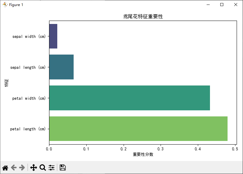
5. 可视化特征重要性
6. (选做)尝试调整n_estimators和max_depth观察准确率变化

# 导入模块
import pandas as pd
from sklearn.datasets import load_iris
from sklearn.decomposition import PCA
from sklearn.model_selection import train_test_split
from sklearn.ensemble import RandomForestClassifier
from sklearn.metrics import accuracy_score, classification_report, confusion_matrix
import matplotlib.pyplot as plt
import seaborn as sns

plt.rcParams['font.sans-serif'] = ['SimHei']
plt.rcParams['axes.unicode_minus'] = False

# 获取数据
iris = load_iris()

# 特征值和目标值
x = iris.data
y = iris.target

# 划分数据集
x_train, x_test, y_train, y_test = train_test_split(x, y, test_size=0.3, random_state=42)

# 训练随机森林模型
rf = RandomForestClassifier(n_estimators=100, max_depth=3)
rf.fit(x_train, y_train)

# 预测
y_pred = rf.predict(x_test)
# 模型评估
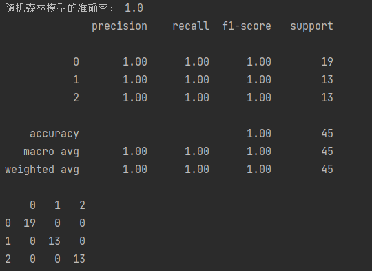
print('随机森林模型的准确率：', accuracy_score(y_test, y_pred))

# 分类评估报告
ret = classification_report(y_test, y_pred)
print(ret)

# 混淆矩阵
cm = confusion_matrix(y_test, y_pred)
print(pd.DataFrame(cm))

# 可视化特征的重要性
importances = rf.feature_importances_
feat_df = pd.DataFrame({'特征': iris.feature_names, '重要性': importances})
feat_df.sort_values(by='重要性', ascending=True, inplace=True)

plt.figure(figsize=(8, 5))
sns.barplot(x='重要性', y='特征', hue='特征', data=feat_df, palette='viridis')
plt.title("鸢尾花特征重要性")
plt.xlabel("重要性分数")
plt.ylabel("特征")
plt.tight_layout()
plt.show()

任务目标‌：

使用随机森林处理类别不平衡的信用卡欺诈检测问题

‌数据集‌：

Kaggle信用卡欺诈数据集(https://www.kaggle.com/mlg-ulb/creditcardfraud)

‌要求步骤‌：

1. 加载信用卡交易数据(注意数据高度不平衡)
2. 标准化Amount特征，Time特征可删除
3. 使用分层抽样划分训练集/测试集
4. 创建随机森林分类器(class_weight='balanced')
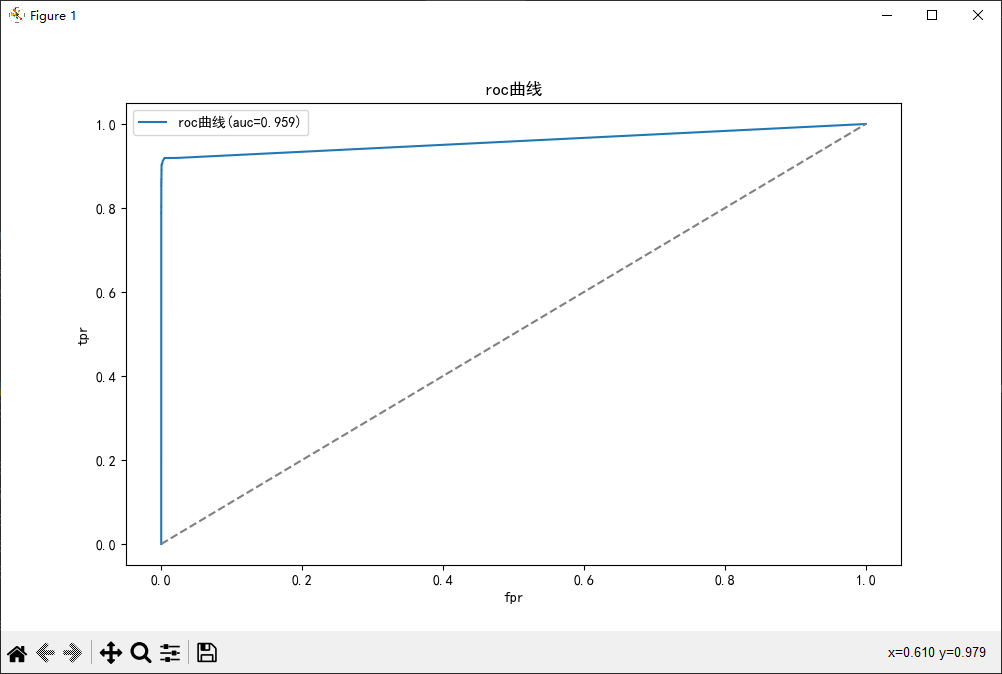
5. 评估模型(使用精确率、召回率、F1、AUC-ROC)
6. (选做)使用SMOTE过采样处理类别不平衡

import numpy as np
from sklearn.datasets import load_iris
from sklearn.decomposition import PCA
from sklearn.model_selection import train_test_split
from sklearn.ensemble import AdaBoostClassifier, GradientBoostingClassifier
from sklearn.tree import DecisionTreeClassifier
from sklearn.metrics import accuracy_score
import matplotlib.pyplot as plt

plt.rcParams['font.sans-serif'] = ['SimHei']
plt.rcParams['axes.unicode_minus'] = False

# 获取数据集
iris = load_iris()

# 特征值和目标值
x = iris.data
y = iris.target

# 降维 可视化
pca = PCA(n_components=2)  # 转换为2维数据
# 调用转换函数 进行转换
x = pca.fit_transform(x)

# 划分数据集
x_train, x_test, y_train, y_test = train_test_split(x, y, test_size=0.3, random_state=42)

# AdaBoost模型
ab = AdaBoostClassifier(
    estimator=DecisionTreeClassifier(max_depth=1),
    n_estimators=50,
    learning_rate=1.0,
    random_state=42
)
# 模型训练
ab.fit(x_train, y_train)

# 模型预测
y_pred = ab.predict(x_test)

# 模型评估
print('AdaBoost模型的准确率：', accuracy_score(y_test, y_pred))

# Gradient Boosting 模型
gb = GradientBoostingClassifier(
    n_estimators=100,
    learning_rate=0.1
)
# 模型训练
gb.fit(x_train, y_train)
# 模型预测
y_pred = gb.predict(x_test)
# 模型评估
print('Gradient Boosting模型准确率:', accuracy_score(y_test, y_pred))

# 创建网格点
x_min, x_max = x[:, 0].min() - 1, x[:, 0].max() + 1
y_min, y_max = x[:, 1].min() - 1, x[:, 1].max() + 1

# x轴和y轴
xx, yy = np.meshgrid(np.arange(x_min, x_max, 0.02),
                     np.arange(y_min, y_max, 0.02))

# 观测每个点
z_ab = ab.predict(np.c_[xx.ravel(), yy.ravel()])
z_gb = gb.predict(np.c_[xx.ravel(), yy.ravel()])

# 绘制图
z_ab = z_ab.reshape(xx.shape)
z_gb = z_gb.reshape(xx.shape)
fig, axs = plt.subplots(1, 2, figsize=(10, 6))
axs[0].contourf(xx, yy, z_ab, alpha=0.5)  # Z 要求需要和xx的样式shape相同
axs[1].contourf(xx, yy, z_gb, alpha=0.5)

axs[0].scatter(x[:, 0], x[:, 1],
               s=20,  # 字体大小
               c=y,  # 使用真实类别决定数据点的颜色
               edgecolors='k'  # 点的边缘颜色是黑色
               )
axs[1].scatter(x[:, 0], x[:, 1],
               s=20,  # 字体大小
               c=y,  # 使用真实类别决定数据点的颜色
               edgecolors='k'  # 点的边缘颜色是黑色
               )
axs[0].set_title('AdaBoost决策边界')
axs[1].set_title('Gradient Boosting决策边界')
axs[0].set_xlabel('主要成分1')
axs[0].set_ylabel('主要成分2')
axs[1].set_xlabel('主要成分1')
axs[1].set_ylabel('主要成分2')
plt.tight_layout()
plt.show()