k-means聚类算法

一. 聚类的定义

聚类能够将相似的样本尽量归入同一类，将不相似的样本归入不同的类，是一种无监督的机器学习算法。其中相似度的评价标准是人为制定的，一般情况下用欧式距离来衡量相似度。

二. k-means算法

k-means算法的伪代码如下：

create k points for starting centroids (often randomly)
while any point has changed cluster assignment
    for every point in our dataset:
        for every centroid
            calculate the distance between the centroid and point
        assign the point to the cluster with the lowest distance
    for every cluster calculate the mean of the points in that cluster
        assign the centroid to the mean

该算法可能收敛到局部最小值，但是可以通过后续处理来提高聚类性能。例如，可以通过SSE（Sum of Squared Error，误差平方和）值来对k-means的聚类结果进行调整，其中拆分和合并的方法如下：
拆分：对SSE值最大的类进行聚类，把它拆分成2个新的类。因为拆分之后多了一个类，所以还需要进行拆分之后还需要进行合并；
合并：有两种方法，合并两个最近的质心，或者合并两个合并后SSE值增幅最小的质心；

三. Bisecting k-means算法

除了上述的后续处理方法外，Bisecting k-means算法也可以很好地解决收敛到局部最小值的问题。
Bisecting k-means算法的伪代码如下：

start with all the points in one cluster
while the number of clusters is less than k
    for every cluster
        measure total error
        perform k-means clustering with k=2 on the given cluster
        measure total error after k-means has split the cluster in two
    choose the cluster split that gives the lowest error and commit this split

四. 实验代码

import numpy
import matplotlib.pyplot as plt

inf = 1e30

def load_data(file_path):
    data = []
    fr = open(file_path)
    for line in fr.readlines():
        arr = line.split('\t')
        data.append(((float)(arr[0]), (float)(arr[1])))
    return numpy.mat(data)

def dist_eclud(a, b):
    return numpy.sqrt(numpy.sum(numpy.power(a - b, 2)))

def rand_cents(data, k):
    dim = data.shape[1]
    cents = numpy.zeros((k, dim), dtype = "float32")
    for i in range(dim):
        min_i = min(data[:, i])
        range_i = float(max(data[:, i]) - min_i)
        cents[:, i] = min_i + range_i * numpy.random.rand(k)
    return cents

def kmeans(data, k, dist_meas = dist_eclud, cents_meas = rand_cents):
    n = data.shape[0]
    cluster_assment = numpy.mat(numpy.zeros((n, 2)))
    cents = cents_meas(data, k)
    cluster_changed = True
    while cluster_changed:
        cluster_changed = False
        for i in range(n):
            min_dist = inf
            min_index = -1
            for j in range(k):
                tmp_dis = dist_meas(cents[j, :], data[i, :])
                if tmp_dis < min_dist:
                    min_dist = tmp_dis
                    min_index = j
            if cluster_assment[i, 0] != min_index:
                cluster_changed = True
            cluster_assment[i, :] = min_index, min_dist ** 2
        # print cents
        for i in range(k):
            pts_in_clust = data[numpy.nonzero(cluster_assment[:, 0].A == i)[0]]
            cents[i, :] = numpy.mean(pts_in_clust, axis = 0)
    return cents, cluster_assment

def bikmeans(data, k, dist_meas = dist_eclud):
    n = data.shape[0]
    cluster_assment = numpy.mat(numpy.zeros((n, 2)))
    cent0 = numpy.mean(data, axis = 0).tolist()[0]
    cent_list = [cent0]
    for i in range(n):
        cluster_assment[i, 1] = dist_meas(numpy.mat(cent0), data[i, :]) ** 2
    while (len(cent_list) < k):
        min_sse = inf
        for i in range(len(cent_list)):
            pts_in_clust = data[numpy.nonzero(cluster_assment[:, 0].A == i)[0], :]
            new_cents, split_cluster_assment = kmeans(pts_in_clust, 2, dist_meas)
            sse_split = sum(split_cluster_assment[:, 1])
            sse_not_split = sum(cluster_assment[numpy.nonzero(cluster_assment[:, 0].A != i)[0], 1])
            print 'sse_split & sse_not_split:', sse_split, sse_not_split
            if (sse_split + sse_not_split) < min_sse:
                best_cent_to_split = i
                best_new_cents = new_cents
                best_cluster_assment = split_cluster_assment
                min_sse = sse_split + sse_not_split
        best_cluster_assment[numpy.nonzero(best_cluster_assment[:, 0].A == 1)[0], 0] = len(cent_list)
        best_cluster_assment[numpy.nonzero(best_cluster_assment[:, 0].A == 0)[0], 0] = best_cent_to_split
        print 'the best cent to split:', best_cent_to_split
        print 'the len of best cluster assment:', len(best_cluster_assment)
        cent_list[best_cent_to_split] = best_new_cents[0, :]
        cent_list.append(best_new_cents[1, :])
        cluster_assment[numpy.nonzero(cluster_assment[:, 0].A == best_cent_to_split)[0], :] = best_cluster_assment
    return cent_list, cluster_assment

def plot(data, cents, cluster_assment):
    color = ['red', 'blue', 'green', 'yellow']
    fig = plt.figure()
    ax = fig.add_subplot(111)

    for i in range(len(cents)):
        pts_in_clust = data[numpy.nonzero(cluster_assment[:, 0].A == i)[0]]
        ax.scatter(pts_in_clust[:, 0], pts_in_clust[:, 1], s = 30, c = color[i])
        ax.scatter(cents[i][0], cents[i][1], s = 100, c = color[i], marker = 'v')

    plt.xlabel('X')
    plt.ylabel('Y')
    plt.show()

if __name__ == "__main__":
    numpy.random.seed(1)
    data = load_data('data.txt')

    cents0, cluster_assment0 = kmeans(data, 4)
    plot(data, cents0, cluster_assment0)

    cents1, cluster_assment1 = bikmeans(data, 4)
    plot(data, cents1, cluster_assment1)

五. 实验数据

data.txt

1.658985    4.285136
-3.453687   3.424321
4.838138    -1.151539
-5.379713   -3.362104
0.972564    2.924086
-3.567919   1.531611
0.450614    -3.302219
-3.487105   -1.724432
2.668759    1.594842
-3.156485   3.191137
3.165506    -3.999838
-2.786837   -3.099354
4.208187    2.984927
-2.123337   2.943366
0.704199    -0.479481
-0.392370   -3.963704
2.831667    1.574018
-0.790153   3.343144
2.943496    -3.357075
-3.195883   -2.283926
2.336445    2.875106
-1.786345   2.554248
2.190101    -1.906020
-3.403367   -2.778288
1.778124    3.880832
-1.688346   2.230267
2.592976    -2.054368
-4.007257   -3.207066
2.257734    3.387564
-2.679011   0.785119
0.939512    -4.023563
-3.674424   -2.261084
2.046259    2.735279
-3.189470   1.780269
4.372646    -0.822248
-2.579316   -3.497576
1.889034    5.190400
-0.798747   2.185588
2.836520    -2.658556
-3.837877   -3.253815
2.096701    3.886007
-2.709034   2.923887
3.367037    -3.184789
-2.121479   -4.232586
2.329546    3.179764
-3.284816   3.273099
3.091414    -3.815232
-3.762093   -2.432191
3.542056    2.778832
-1.736822   4.241041
2.127073    -2.983680
-4.323818   -3.938116
3.792121    5.135768
-4.786473   3.358547
2.624081    -3.260715
-4.009299   -2.978115
2.493525    1.963710
-2.513661   2.642162
1.864375    -3.176309
-3.171184   -3.572452
2.894220    2.489128
-2.562539   2.884438
3.491078    -3.947487
-2.565729   -2.012114
3.332948    3.983102
-1.616805   3.573188
2.280615    -2.559444
-2.651229   -3.103198
2.321395    3.154987
-1.685703   2.939697
3.031012    -3.620252
-4.599622   -2.185829
4.196223    1.126677
-2.133863   3.093686
4.668892    -2.562705
-2.793241   -2.149706
2.884105    3.043438
-2.967647   2.848696
4.479332    -1.764772
-4.905566   -2.911070

六. 实验结果

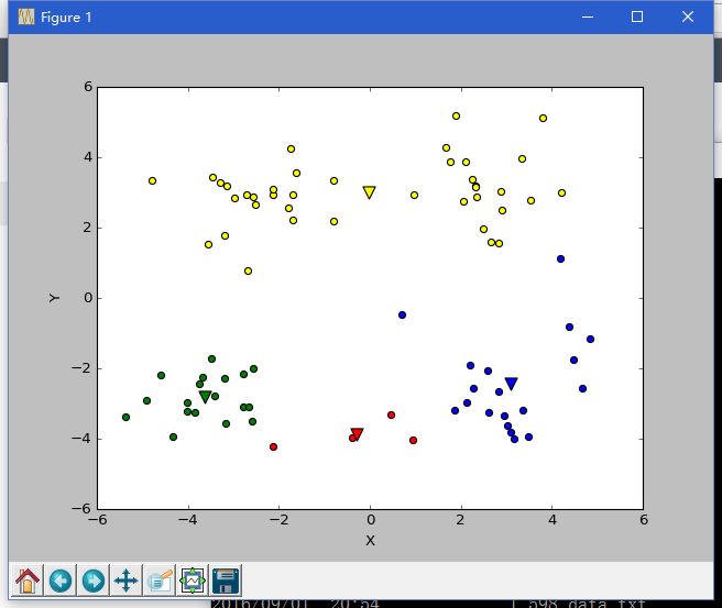
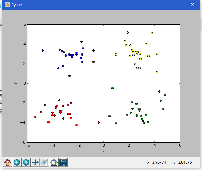
由下图可以看出，在这种情况下，k-means算法收敛到了局部最小值，而Bisecting k-means算法避免了这个问题

如有错误请指正