图机器学习基础知识——CS224W（03-nodeemb）

CS224W: Machine Learning with Graphs

Stanford / Winter 2021

03-nodeemb

• Why Embedding ?

  Task: map nodes into an embedding space

  • Similarity of embeddings between nodes indicates their similarity in the network

  • Encode network information

  • Potentially used for many downstream predictions

Node Embeddings: Encoder and Decoder

ENC and DEC

• Assume we have a graph $G$

  • $V$ is the vertex set

  • $A$ is the adjacency matrix (assume binary)

  • For simplicity: no node features or extra information is used

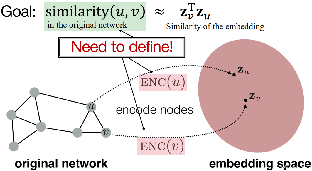
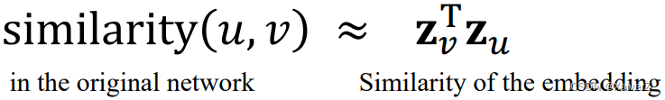
• Goal: Encode nodes so that similarity in the embedding space (e.g. dot product) approximates similarity in the graph

  

• How to learn node embeddings ?

  • Encoders (ENC) maps from nodes to embeddings

  • Define a node similarity function (i.e. a measure of similarity in the original network)

  • Decoder (DEC) maps from embeddings to the similarity score

  • Optimiza the parameters of the encoder so that

    

• Two Key Components

  • Encoder: maps each node to a low-dimensional vector

    $$\mathrm{ENC}(v)={\mathbf{z}}_v$$

  • Decoder (Similarity Function): specifies how the relationships in vector space map to the relationship in the original network (向量空间中的关系如何映射成原图上的关系)

    $$\mathrm{similarity}(u,v)\approx {\mathbf{z}}_v^{\mathrm{T}}{\mathbf{z}}_u$$

• Note on Node Embeddings

  • This is unsupervised/self-supervised way of learning node embeddings

    • Not utilizing node labels

    • Not utilizing node features

    • Goal is to directly estimate a set of coordinates (e.g. the embedding) of a node so that some aspect of the network structure is preserved

  • These embeddings are task independent

    • They are not trained for a specific task but can be used for any task

“Shallow” Encoding

“Shallow” Encoding

• Simplest encoding approach: Encoder is just an embedding-lookup

  $$\mathrm{ENC}(v)={\mathbf{z}}_v=\mathbf{Z}\cdot v$$
  $\mathbf{Z}\in {\mathbb{R}}^{d\times |\mathcal{V}|}$: matrix, each column is a node embedding (exactly what we learn and optimize); $v\in {\mathbb{I}}^{|\mathcal{V}|}$: indicator vector, all zeroes except a one in column indicating node $v$

  

Random Walk Approaches for Node Embeddings

Shallow Embedding

Given a graph and a starting point, we select a neighbor of it at random, and move to this neighbor; then we select a neighbor of this point at random, and move to it, etc. The (random) sequence of points visited this way is a random walk on the graph

Random Walk可以看作是一个算法框架，描述了Random Walk基本的算法思路，具体的算法实现（主要是随机游走的策略部分）可以有很多种，例如DeepWalk等

• Notation

  • Vector $z_u$

    • The embedding of node $u$

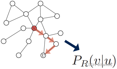
  • Probability $P(v|z_u)$

    • The (predicted) probability of visiting node $v$ on random walks starting from node $u$ (从节点$u$出发使用random walks访问到节点$v$的概率)

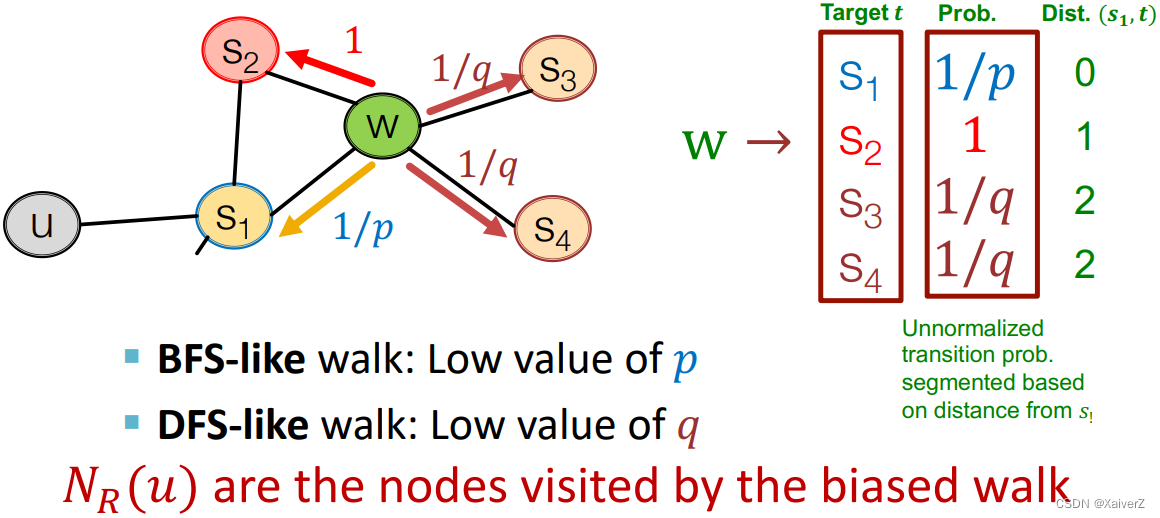
  • $N_R(u)$: Neighborhood of $u$ obtained by some random walk strategy $R$ ($u$在一次随机游走中访问过的节点)

• Random-Walk Embeddings

  • 可以认为${\mathbf{z}}_u^{\mathrm{T}}{\mathbf{z}}_v$约等于$u$和$v$同时出现在一次随机游走上的概率

  • Estimate probability of visiting node $v$ on a random walk starting from node $u$ using some random walk strategy $R$

    

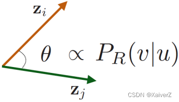
  • Optimize embeddings to encode these random walk statistics (Similarity in embedding space (Here: dot product=cos(θ)) encodes random walk “similarity”)

    

• Random Walk Optimization

  • Given $G=(V,E)$

  • Goal: To learn a mapping $f:u\to R^d:f(u)=z_u$

  • Run short fixed-length random walks starting from each node $u$ in the graph using some random walk strategy $R$

  • For each node $u$ collect $N_R(u)$, the multiset of nodes visited on random walks starting from $u$

  • Optimize embeddings according to: Given node $u$, predict its neighbors $N_R(u)$

  • Log-likelihood objective

    $$\underset{f}{\max }\sum _{u\in V}\log \mathrm{P}\left(N_{\mathrm{R}}(u)\mid {\mathbf{z}}_u\right)$$
    $N_{\mathrm{R}}(u)$ is the neighborhood of node $u$ by strategy $R$

  • Equivalently, objective function can be rewrited as

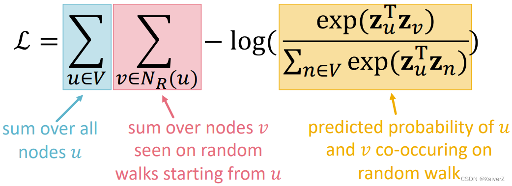
    $$\mathcal{L}=\sum _{u\in V}\sum _{v\in N_R(u)}-\log \left(P\left(v\mid {\mathbf{z}}_u\right)\right)$$
    Optimize embeddings $z_u$ to maximize the likelihood of random walk co-occurrences (最大化在random walk中同时出现的似然概率)

  • Parameterize $P(v|z_u)$ using softmax (We want node $v$ to be most similar to node $u$ (out of all nodes $n$))

    $$P\left(v\mid {\mathbf{z}}_u\right)=\frac{\exp \left({\mathbf{z}}_u^{\mathrm{T}}{\mathbf{z}}_v\right)}{{\sum }_{n\in V}\exp \left({\mathbf{z}}_u^{\mathrm{T}}{\mathbf{z}}_n\right)}$$

  • Then we get the final objective, which uses to minimize （using SGD optimizer）

    $$\mathcal{L}=\sum _{u\in V}\sum _{v\in N_R(u)}-\log \left(\frac{\exp \left({\mathbf{z}}_u^{\mathrm{T}}{\mathbf{z}}_v\right)}{{\sum }_{n\in V}\exp \left({\mathbf{z}}_u^{\mathrm{T}}{\mathbf{z}}_n\right)}\right)$$

    

Negative Sampling

负采样

• 上述目标函数计算softmax时间复杂度过高，$O(|V{|}^2)$，可用层次化softmax解决，也可以用这里说的Negative Sampling

• 简单来说，不对所有节点作softmax分母的加和操作，而是采样一些负样本进行加和

  $$\log \left(\frac{\exp \left({\mathbf{z}}_u^{\mathrm{T}}{\mathbf{z}}_v\right)}{{\sum }_{n\in V}\exp \left({\mathbf{z}}_u^{\mathrm{T}}{\mathbf{z}}_n\right)}\right)\approx \log \left(\sigma \left({\mathbf{z}}_u^{\mathrm{T}}{\mathbf{z}}_v\right)\right)-\sum _{i=1}^k\log \left(\sigma \left({\mathbf{z}}_u^{\mathrm{T}}{\mathbf{z}}_{n_i}\right)\right),n_i\sim P_V$$
  Instead of normalizing w.r.t. all nodes, just normalize against $k$ random “negative samples” $n_i$

  • Sample $k$ negative nodes each with prob. proportional to its degree (以节点的度为概率参考值，度越大，选择作为负样本的概率越大)

  • Two consideration for $k$ (#negative samples)

    • Higher $k$ gives more robust estimates

    • Higher $k$ corresponds to higher bias on negative events

    • In practice, $k=5-20$

• Why is the approximation valid ?

  Paper : word2vec Explained: Deriving Mikolov et al.’s Negative-Sampling Word-Embedding Method

  Why ???

  • Technically, this is a different objective. But Negative Sampling is a form of Noise Contrastive Estimation (NCE) which approx. maximizes the log probability of softmax

  • New formulation corresponds to using a logistic regression (sigmoid func.) to distinguish the target node $v$ from nodes $n_i$ sampled from background distribution $P_v$

Node2Vec

Node2Vec

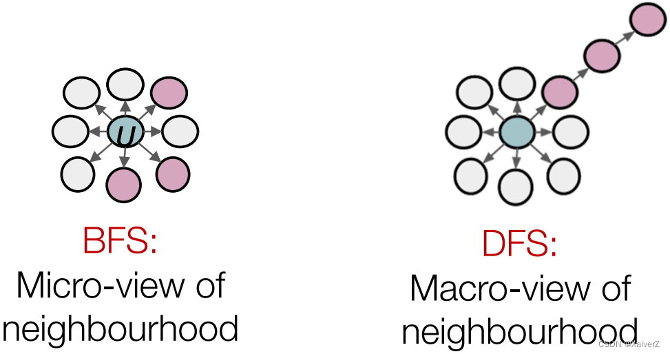
• Key Idea: use flexible, biased random walks that can trade off between local and global views of the network

  

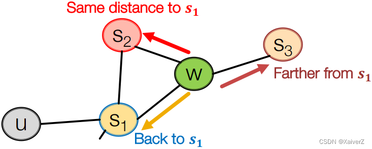
• Biased $2^{nd}$-order Random Walks

  • Biased fixed-length random walk $R$ that given a node $u$ generates neighborhood $N_R(u)$

  • Two parameters

    • Return parameter $p$: Return back to the previous node

    • In-out parameter $q$: Moving outwards (DFS) vs. inwards (BFS). Intuitively, $q$ is the ratio of BFS vs. DFS

  • Rnd. walk just traversed edge $(s_1,w)$ and is now at $w$, neighbors of $w$ can only be (Idea: Remember where the walk came from)

    

    

• Algorithm

  Linear-time complexity

  All 3 steps are individually parallelizable

  • Compute random walk probabilities

  • Simulate $r$ random walks of length $l$ starting from each node $u$

  • Optimize the node2vec objective using SGD

Other Random Walk Ideas

Different kinds of biased random walks

Paper : metapath2vec: Scalable Representation Learning for Heterogeneous Networks

Paper : Watch Your Step: Learning Node Embeddings via Graph Attention

Different kinds of biased random walks

Alternative optimization schemes

Paper : LINE: Large-scale Information Network Embedding

Alternative optimization schemes

Network preprocessing techniques

Paper : struc2vec: Learning Node Representations from Structural Identity

Paper : HARP: Hierarchical Representation Learning for Networks

Network preprocessing techniques

• No one method wins in all cases

Paper : Graph Embedding Techniques, Applications, and Performance: A Survey

• In general: Must choose definition of node similarity that matches your application!

Embedding Entire Graphs

Embedding Entire Graphs

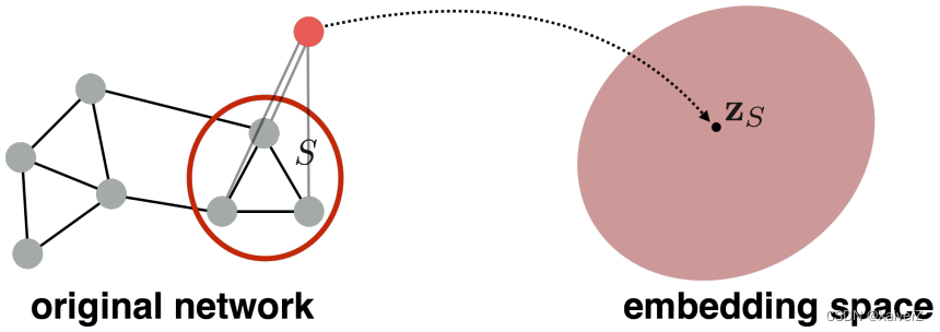
• Goal: Embed a subgraph or an entire graph $G$ to $z_G$

Approach 1

Paper : Convolutional Networks on Graphs for Learning Molecular Fingerprints

Approach 1

• Algorithm

  • Run a standard graph embedding technique on the (sub)graph $G$

  • Then just sum (or average) the node embeddings in the (sub)graph $G$ (简单平均或加和图中所有节点的embedding vector)

    $${\mathbf{Z}}_{\mathbf{G}}=\sum _{v\in G}{Z}_v$$

Approach 2

Paper : GATED GRAPH SEQUENCE NEURAL NETWORKS

Approach 2

• Algorithm

  • Introduce a “virtual node” to represent the (sub)graph and run a standard graph embedding technique （引入一个“虚拟节点”，连接需要embedding的子图区域中的所有节点，而后进行Node Embedding，以该虚拟节点的embedding vector代表子图区域的embedding vector）

    

Approach 3: Anonymous Walk Embeddings

Paper : Anonymous Walk Embeddings

Approach 3: Anonymous Walk Embeddings

• States in anonymous walks correspond to the index of the first time we visited the node in a random walk(核心算法与Random Walk一致，只不过节点是“匿名”的，如下图所示)

  

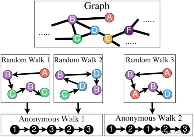
  • Agnostic to the identity of the nodes visited (hence anonymous)

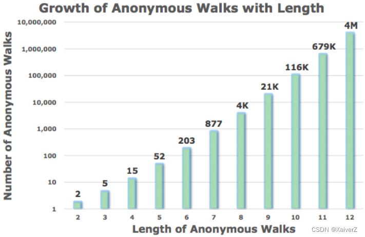
• Number of Walks Grows

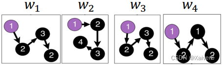
  • There are 5 anonymous walks $w_i$ of length 3

    $$w_1=111,w_2=112,w_3=121,w_4=122,w_5=123$$

  

Simple Use of Anonymous Walks

Simple Use of Anonymous Walks

• Key Idea: Simulate anonymous walks $w_i$ of $l$ steps and record their counts. Represent the graph as a probability distribution over these walks

• For example

  将Graph Embedding表示为各个匿名随机游走序列出现的频率向量

  • Set $l=3$

  • Generate independently a set of $m$ random walks

    • Deciding $m$: We want the distribution to have error of more than $\epsilon$ with prob. less than $\delta$ (误差超过$\epsilon$的概率小于$\delta$)

      $$m=\left[\frac{2}{{\epsilon }^2}\left(\log \left(2^{\eta }-2\right)-\log (\delta )\right)\right]$$
      $\eta$为长为$l$的随机游走所有可能的匿名序列组合数量

  • Then we can represent the graph as a 5-dim vector (since there are 5 anonymous walks $w_i$ of length 3)

  • $Z_G[i]$: the probability of anonymous walk $w_i$ in $G$

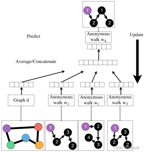
Learn Walk Embeddings

Learn Walk Embeddings

• Key Idea: Rather than simply represent each walk by the fraction of times it occurs, we learn embedding $z_i$ of anonymous walk $w_i$

  • In the meantime, we also learn a graph embedding $Z_G$ together with all the anonymous walk embeddings $z_i$ （学习每个$w_i$的Embedding，顺便把图表示$Z_G$也学了）

• Algorithm

  • Sample anonymous random walks

    

  • Learn to predict walks that co-occur in Δ-size window (e.g. predict $w_2$ given $w_1,w_3$ if $\Delta =1$, something like Skip-gram)

  • Objective

    max ⁡ Z , d 1 T ∑ t = Δ T − Δ log ⁡ P ( w t ∣ { w t − Δ , … , w t + Δ , z G } ) \max _{\mathrm{Z}, \mathrm{d}} \frac{1}{T} \sum_{t=\Delta}^{T-\Delta} \log P\left(w_{t} \mid\left\{w_{t-\Delta}, \ldots, w_{t+\Delta}, \boldsymbol{z}_{\boldsymbol{G}}\right\}\right) Z,dmax​T1​t=Δ∑T−Δ​logP(wt​∣{wt−Δ​,…,wt+Δ​,zG​})

    • 我们可以用softmax去建模log-prob条件概率，并用一个函数$y(\cdot )$去整合信息

      P ( w t ∣ { w t − Δ , … , w t + Δ , z G } ) = exp ⁡ ( y ( w t ) ) ∑ i = 1 η exp ⁡ ( y ( w i ) ) P\left(w_{t} \mid\left\{w_{t-\Delta}, \ldots, w_{t+\Delta}, \boldsymbol{z}_{\boldsymbol{G}}\right\}\right)=\frac{\exp \left(y\left(w_{t}\right)\right)}{\sum_{i=1}^{\eta} \exp \left(y\left(w_{i}\right)\right)} P(wt​∣{wt−Δ​,…,wt+Δ​,zG​})=∑i=1η​exp(y(wi​))exp(y(wt​))​

      $$y\left(w_t\right)=b+U\cdot \left(\mathrm{cat}\left(\frac{1}{2\Delta }\sum _{i=-\Delta }^{\Delta }{z}_i,{\mathbf{z}}_{\mathbf{G}}\right)\right)$$
      其中$\mathrm{cat}\left(\frac{1}{2\Delta }{\sum }_{i=-\Delta }^{\Delta }{Z}_i,{\mathbf{Z}}_G\right)$表示以$w_t$为中心的窗口内随机游走embedding的加和平均，再拼接上图Embedding$Z_G$。$b\in \mathbb{R},U\in {\mathbb{R}}^D$都是可学习参数。$y(\cdot )$表示一个线性层