ML算法整理（一）线性回归与梯度下降 python实现

回归算法

以下均为自己看视频做的笔记，自用，侵删！

转自https://www.cnblogs.com/douzujun/p/8370657.html

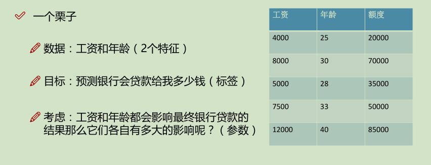
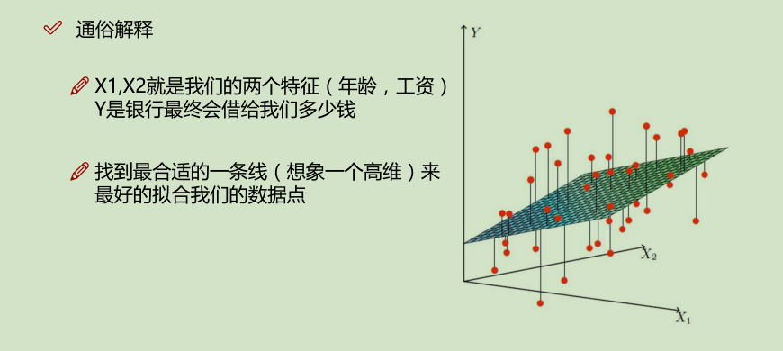
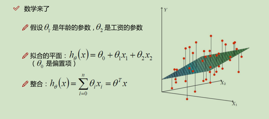
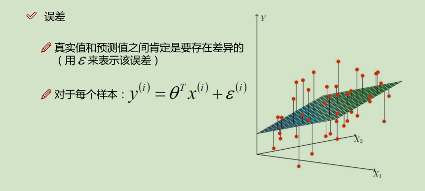
一、线性回归

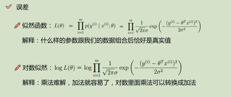
θ是bias(偏置项)

线性回归算法代码实现

# coding: utf-8
​
get_ipython().run_line_magic('matplotlib', 'inline')
import matplotlib.pylab as plt
import numpy as np
from sklearn import datasets
​
# $h_{\theta}(x)=\theta_0+\theta_1x_1+\theta_2x_2$
# 
# 将 $\theta_0$ 放到权重项上来,将 $\theta_0$ = 1
​
class LinearRegression():
    def __init__(self):
        self.w = None
        
    def fit(self, X, y):
        # Insert constant ones for bias weights
        print("first:", X.shape)
        # 在第0项，插入 1，让x0项为1
        X = np.insert(X, 0, 1, axis=1)
        print("second:", X.shape)
        # inv(): 对当前值取逆， dot()：矩阵计算
        X_ = np.linalg.inv(X.T.dot(X))
        # 算出来 最好的 一组参数 theta
        self.w = X_.dot(X.T).dot(y)
    
    def predict(self, X):
        # Insert constant ones for bias weights
        X = np.insert(X, 0, 1, axis=1)
        y_pred = X.dot(self.w)
        return y_pred
​
def mean_squared_error(y_true, y_pred):
    mse = np.mean(np.power(y_true - y_pred, 2))
    return mse
​
def main():
    # load the diabetes dataset
    diabetes = datasets.load_diabetes()
    
    # Use only one feature
    X = diabetes.data[: , np.newaxis, 2]
    print(X.shape)
    # split the data into training/testing sets
    x_train, x_test = X[:-20], X[-20:]
    
    # Split the targets into training/testing sets
    y_train, y_test = diabetes.target[:-20], diabetes.target[-20:]
    
    clf = LinearRegression()
    clf.fit(x_train, y_train)
    y_pred = clf.predict(x_test)
    
    # Print the mean squared error
    print("Mean Squared Error:", mean_squared_error(y_test, y_pred))
    
    # Plot the results
    plt.scatter(x_test[: , 0], y_test, color='black')
    plt.plot(x_test[:, 0], y_pred, color="blue", linewidth=3)
    plt.show()
​
main()

 

具体实现：

可以我用jupyter写的版本（格式会好看点）：https://douzujun.github.io/page/%E6%95%B0%E6%8D%AE%E6%8C%96%E6%8E%98%E7%AC%94%E8%AE%B0/5-%E5%9B%9E%E5%BD%92%E7%AE%97%E6%B3%95/Code/%E9%80%BB%E8%BE%91%E5%9B%9E%E5%BD%92%E4%B8%8E%E6%A2%AF%E5%BA%A6%E4%B8%8B%E9%99%8D_GradientDescent.html

实验数据下载：https://github.com/douzujun/douzujun.github.io/tree/master/page/%E6%95%B0%E6%8D%AE%E6%8C%96%E6%8E%98%E7%AC%94%E8%AE%B0/5-%E5%9B%9E%E5%BD%92%E7%AE%97%E6%B3%95/Code

# coding: utf-8
# In[3]:
get_ipython().run_line_magic('matplotlib', 'inline')
import pandas as pd
import matplotlib.pylab as plt
# Read data from csv
pga = pd.read_csv("pga.csv")
# Normalize the data 归一化值 (x - mean) / (std)
pga.distance = (pga.distance - pga.distance.mean()) / pga.distance.std()
pga.accuracy = (pga.accuracy - pga.accuracy.mean()) / pga.accuracy.std()
print(pga.head())
plt.scatter(pga.distance, pga.accuracy)
plt.xlabel('normalized distance')
plt.ylabel('normalized accuracy')
plt.show()
# ### accuracy = $\theta_1$ $distance_i$ + $\theta_0$ + $\alpha$
# - $\theta_0$是bias
# In[4]:
# accuracyi=θ1distancei+θ0+ϵ
from sklearn.linear_model import LinearRegression
import numpy as np
# We can add a dimension to an array by using np.newaxis
print("Shape of the series:", pga.distance.shape)
print("Shape with newaxis:", pga.distance[:, np.newaxis].shape)
# The X variable in LinearRegression.fit() must have 2 dimensions
lm = LinearRegression()
lm.fit(pga.distance[:, np.newaxis], pga.accuracy)
theta1 = lm.coef_[0]
print (theta1)
# ### accuracy = $\theta_1$ $distance_i$ + $\theta_0$ + $\alpha$
# - $\theta_0$是bias
# - #### 没有用梯度下降来求代价函数
# In[9]:
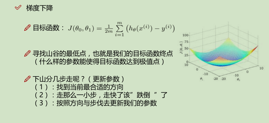
# The cost function of a single variable linear model
# 单变量 代价函数
def cost(theta0, theta1, x, y):
    # Initialize cost
    J = 0
    # The number of observations
    m = len(x)
    # Loop through each observation
    # 通过每次观察进行循环
    for i in range(m):
        # Compute the hypothesis 
        # 计算假设
        h = theta1 * x[i] + theta0
        # Add to cost
        J += (h - y[i])**2
    # Average and normalize cost
    J /= (2*m)
    return J
# The cost for theta0=0 and theta1=1
print(cost(0, 1, pga.distance, pga.accuracy))
theta0 = 100
theta1s = np.linspace(-3,2,100)
costs = []
for theta1 in theta1s:
    costs.append(cost(theta0, theta1, pga.distance, pga.accuracy))
plt.plot(theta1s, costs)
plt.show()
# In[6]:
import numpy as np
from mpl_toolkits.mplot3d import Axes3D
# Example of a Surface Plot using Matplotlib
# Create x an y variables
x = np.linspace(-10,10,100)
y = np.linspace(-10,10,100)
# We must create variables to represent each possible pair of points in x and y
# ie. (-10, 10), (-10, -9.8), ... (0, 0), ... ,(10, 9.8), (10,9.8)
# x and y need to be transformed to 100x100 matrices to represent these coordinates
# np.meshgrid will build a coordinate matrices of x and y
X, Y = np.meshgrid(x,y)
#print(X[:5,:5],"\n",Y[:5,:5])
# Compute a 3D parabola 
Z = X**2 + Y**2 
# Open a figure to place the plot on
fig = plt.figure()
# Initialize 3D plot
ax = fig.gca(projection='3d')
# Plot the surface
ax.plot_surface(X=X,Y=Y,Z=Z)
plt.show()
# Use these for your excerise 
theta0s = np.linspace(-2,2,100)
theta1s = np.linspace(-2,2, 100)
COST = np.empty(shape=(100,100))
# Meshgrid for paramaters 
T0S, T1S = np.meshgrid(theta0s, theta1s)
# for each parameter combination compute the cost
for i in range(100):
    for j in range(100):
        COST[i,j] = cost(T0S[0,i], T1S[j,0], pga.distance, pga.accuracy)
# make 3d plot
fig2 = plt.figure()
ax = fig2.gca(projection='3d')
ax.plot_surface(X=T0S,Y=T1S,Z=COST)
plt.show()
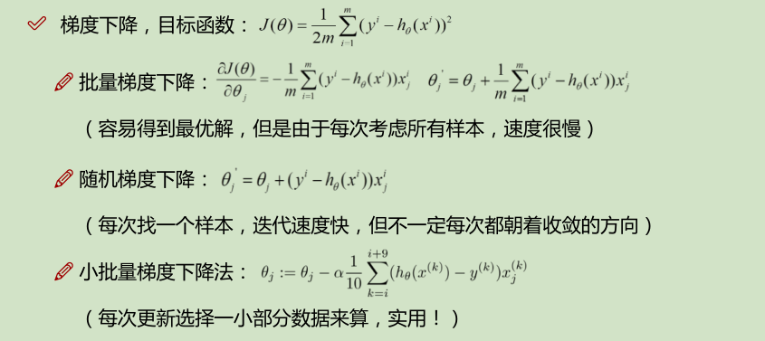
# ### 求导
# In[21]:
# 对 theta1 进行求导
def partial_cost_theta1(theta0, theta1, x, y):
    # Hypothesis
    h = theta0 + theta1*x
    # Hypothesis minus observed times x
    diff = (h - y) * x
    # Average to compute partial derivative
    partial = diff.sum() / (x.shape[0])
    return partial
partial1 = partial_cost_theta1(0, 5, pga.distance, pga.accuracy)
print("partial1 =", partial1)
# 对theta0 进行求导
# Partial derivative of cost in terms of theta0
def partial_cost_theta0(theta0, theta1, x, y):
    # Hypothesis
    h = theta0 + theta1*x
    # Difference between hypothesis and observation
    diff = (h - y)
    # Compute partial derivative
    partial = diff.sum() / (x.shape[0])
    return partial
partial0 = partial_cost_theta0(1, 1, pga.distance, pga.accuracy)
print("partial0 =", partial0)
# ### 梯度下降进行更新
# In[22]:
# x is our feature vector -- distance
# y is our target variable -- accuracy
# alpha is the learning rate
# theta0 is the intial theta0 
# theta1 is the intial theta1
def gradient_descent(x, y, alpha=0.1, theta0=0, theta1=0):
    max_epochs = 1000 # Maximum number of iterations 最大迭代次数
    counter = 0       # Intialize a counter 当前第几次
    c = cost(theta1, theta0, pga.distance, pga.accuracy)  ## Initial cost 当前代价函数
    costs = [c]     # Lets store each update 每次损失值都记录下来
    # Set a convergence threshold to find where the cost function in minimized
    # When the difference between the previous cost and current cost 
    #        is less than this value we will say the parameters converged
    # 设置一个收敛的阈值 (两次迭代目标函数值相差没有相差多少,就可以停止了)
    convergence_thres = 0.000001  
    cprev = c + 10   
    theta0s = [theta0]
    theta1s = [theta1]
    # When the costs converge or we hit a large number of iterations will we stop updating
    # 两次间隔迭代目标函数值相差没有相差多少(说明可以停止了)
    while (np.abs(cprev - c) > convergence_thres) and (counter < max_epochs):
        cprev = c
        # Alpha times the partial deriviative is our updated
        # 先求导, 导数相当于步长
        update0 = alpha * partial_cost_theta0(theta0, theta1, x, y)
        update1 = alpha * partial_cost_theta1(theta0, theta1, x, y)
        # Update theta0 and theta1 at the same time
        # We want to compute the slopes at the same set of hypothesised parameters
        #             so we update after finding the partial derivatives
        # -= 梯度下降，+=梯度上升
        theta0 -= update0
        theta1 -= update1
        
        # Store thetas
        theta0s.append(theta0)
        theta1s.append(theta1)
        
        # Compute the new cost
        # 当前迭代之后，参数发生更新  
        c = cost(theta0, theta1, pga.distance, pga.accuracy)
        # Store updates，可以进行保存当前代价值
        costs.append(c)
        counter += 1   # Count
        
    # 将当前的theta0, theta1, costs值都返回去
    return {'theta0': theta0, 'theta1': theta1, "costs": costs}
print("Theta0 =", gradient_descent(pga.distance, pga.accuracy)['theta0'])
print("Theta1 =", gradient_descent(pga.distance, pga.accuracy)['theta1'])
print("costs =", gradient_descent(pga.distance, pga.accuracy)['costs'])
descend = gradient_descent(pga.distance, pga.accuracy, alpha=.01)
plt.scatter(range(len(descend["costs"])), descend["costs"])
plt.show()

 

 

 

 

Theta0 = 1.4072555867362913e-14
Theta1 = -0.6046983166379609
costs = [0.49746192893401031, 0.46273605725902511, 0.43457636303154484, 0.41174127378146347, 0.39322398105637657, 0.37820804982390627, 0.36603142151620471, 0.3561572235961119, 0.34815009862675572, 0.34165700918356962, 0.33639167228942018, 0.33212193708070803, 0.32865954918055734, 0.32585185048611698, 0.32357504841017987, 0.32172875781523191, 0.32023157499156085, 0.31901748853429884, 0.31803296887350535, 0.31723460813346771, 0.31658720626165587, 0.31606221904396564, 0.31563649957860979, 0.31529127771972282, 0.31501133249393021, 0.31478432100138809, 0.31460023421226618, 0.31445095566451636, 0.3143299036057311, 0.31423174080098198, 0.31415213921193808, 0.31408758917188512, 0.3140352446430773, 0.31399279773376704, 0.31395837694231021, 0.31393046464189178, 0.31390783016773566, 0.31388947555659158, 0.31387459154612474, 0.31386252189420782, 0.31385273444493683, 0.31384479766565831, 0.31383836162051826, 0.31383314254164574, 0.31382891031771304, 0.3138254783482301, 0.31382269531625501, 0.31382043851676622, 0.31381860844654841, 0.31381712441705512, 0.31381592099681721, 0.31381494512654245]