DDPM公式推导（五）

3 Diffusion models and denoising autoencoders

扩散模型可能看起来是一类受限制的潜在变量模型，但它们在实现中允许很大的自由度。必须选择正向过程的方差${\beta }_t$以及逆向过程的模型架构和高斯分布参数化。为了指导我们的选择，我们在扩散模型和去噪分数匹配之间建立了一个新的显式连接（第 3.2 节），从而为扩散模型提供了一个简化的加权变分边界目标（第 3.4 节）。最终，我们的模型设计通过简单性和实证结果得到了证明（第 4 节）。我们的讨论按公式（5）的术语进行分类。

3.1 Forward process and $L_T$

---

我们忽略了通过重参数化可以使前向过程的方差${\beta }_t$变得可学习的事实，而是将它们固定为常数（详见第4节）。因此，在我们的实现中，近似后验分布$q$没有可学习的参数，因此$L_T$在训练过程中是一个常数，可以忽略不计。

3.2 Reverse process and $L_{1:T-1}$

---

现在我们讨论 $p_{\theta }\left({\mathbf{x}}_{t-1}\mid {\mathbf{x}}_t\right)=\mathcal{N}\left({\mathbf{x}}_{t-1};{\mathbf{\mu }}_{\theta }\left({\mathbf{x}}_t,t\right),{\mathbf{\Sigma }}_{\theta }\left({\mathbf{x}}_t,t\right)\right)$ 中对 $1<t\le T$ 的选择。首先，我们将 ${\mathbf{\Sigma }}_{\theta }\left({\mathbf{x}}_t,t\right)={\sigma }_t^2\mathbf{I}$ 设为未训练的时间依赖常数。实验上，${\sigma }_t^2={\beta }_t$ 和 ${\sigma }_t^2={\tilde{\beta }}_t=\frac{1-{\bar{\alpha }}_{t-1}}{1-{\bar{\alpha }}_t}{\beta }_t$ 有类似的结果。第一个选择对于 ${\mathbf{x}}_0\sim \mathcal{N}(0,\mathbf{I})$ 是最优的，而第二个选择对于 ${\mathbf{x}}_0$ 确定为某一个点是最优的。这是对应于坐标单位方差数据的逆过程熵上下界的两个极端选择 [53]。

其次，为了表示均值 ${\mathbf{\mu }}_{\theta }\left({\mathbf{x}}_t,t\right)$，我们提出了一种特定的参数化方法，这种方法的动机来源于对 $L_t$ 的以下分析。对于 $p_{\theta }\left({\mathbf{x}}_{t-1}\mid {\mathbf{x}}_t\right)=\mathcal{N}\left({\mathbf{x}}_{t-1};{\mathbf{\mu }}_{\theta }\left({\mathbf{x}}_t,t\right),{\sigma }_t^2\mathbf{I}\right)$，我们可以写成：
$$L_{t-1}={\mathbb{E}}_q\left[\frac{1}{2{\sigma }_t^2}{\Vert {\tilde{\mathbf{\mu }}}_t\left({\mathbf{x}}_t,{\mathbf{x}}_0\right)-{\mathbf{\mu }}_{\theta }\left({\mathbf{x}}_t,t\right)\Vert }^2\right]+C(8)$$
其中 $C$ 是一个不依赖于 $\theta$ 的常数。因此，我们看到 ${\mathbf{\mu }}_{\theta }$ 最直接的参数化方式是预测前向过程的后验均值 ${\tilde{\mathbf{\mu }}}_t$。但是，我们可以通过将公式 (4) 重参数化为 ${\mathbf{x}}_t\left({\mathbf{x}}_0,\mathbf{ϵ}\right)=\sqrt{{\bar{\alpha }}_t}{\mathbf{x}}_0+\sqrt{1-{\bar{\alpha }}_t}\mathbf{ϵ}$ 对 $\mathbf{ϵ}\sim \mathcal{N}(0,\mathbf{I})$，并应用前向过程的后验公式 (7) 来进一步展开公式 (8)：
$$\begin{array}{rl}{L}_{t-1}-C& ={\mathbb{E}}_{{\mathbf{x}}_0,\mathbf{ϵ}}\left[\frac{1}{2{\sigma }_t^2}{\Vert {\tilde{\mathbf{\mu }}}_t\left({\mathbf{x}}_t\left({\mathbf{x}}_0,\mathbf{ϵ}\right),\frac{1}{\sqrt{{\bar{\alpha }}_t}}\left({\mathbf{x}}_t\left({\mathbf{x}}_0,\mathbf{ϵ}\right)-\sqrt{1-{\bar{\alpha }}_t}\mathbf{ϵ}\right)\right)-{\mathbf{\mu }}_{\theta }\left({\mathbf{x}}_t\left({\mathbf{x}}_0,\mathbf{ϵ}\right),t\right)\Vert }^2\right](9)\\ & ={\mathbb{E}}_{{\mathbf{x}}_0,\mathbf{ϵ}}\left[\frac{1}{2{\sigma }_t^2}{\Vert \frac{1}{\sqrt{{\alpha }_t}}\left({\mathbf{x}}_t\left({\mathbf{x}}_0,\mathbf{ϵ}\right)-\frac{{\beta }_t}{\sqrt{1-{\bar{\alpha }}_t}}\mathbf{ϵ}\right)-{\mathbf{\mu }}_{\theta }\left({\mathbf{x}}_t\left({\mathbf{x}}_0,\mathbf{ϵ}\right),t\right)\Vert }^2\right](10)\end{array}$$

公式（10）揭示了 ${\mathbf{\mu }}_{\theta }$ 必须预测 $\frac{1}{\sqrt{{\alpha }_t}}\left({\mathbf{x}}_t-\frac{{\beta }_t}{\sqrt{1-{\bar{\alpha }}_t}}\mathbf{ϵ}\right)$ 给定 ${\mathbf{x}}_t$。由于 ${\mathbf{x}}_t$ 作为模型的输入是可用的，我们可以选择参数化方式：
$${\mathbf{\mu }}_{\theta }\left({\mathbf{x}}_t,t\right)={\tilde{\mathbf{\mu }}}_t\left({\mathbf{x}}_t,\frac{1}{\sqrt{{\bar{\alpha }}_t}}\left({\mathbf{x}}_t-\sqrt{1-{\bar{\alpha }}_t}{\mathbf{ϵ}}_{\theta }\left({\mathbf{x}}_t\right)\right)\right)=\frac{1}{\sqrt{{\alpha }_t}}\left({\mathbf{x}}_t-\frac{{\beta }_t}{\sqrt{1-{\bar{\alpha }}_t}}{\mathbf{ϵ}}_{\theta }\left({\mathbf{x}}_t,t\right)\right)(11)$$
其中 ${\mathbf{ϵ}}_{\theta }$ 是一个函数逼近器，用于从 ${\mathbf{x}}_t$ 预测 $\mathbf{ϵ}$。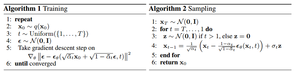采样 ${\mathbf{x}}_{t-1}\sim p_{\theta }\left({\mathbf{x}}_{t-1}\mid {\mathbf{x}}_t\right)$ 相当于计算 ${\mathbf{x}}_{t-1}=\frac{1}{\sqrt{{\alpha }_t}}\left({\mathbf{x}}_t-\frac{{\beta }_t}{\sqrt{1-{\bar{\alpha }}_t}}{\mathbf{ϵ}}_{\theta }\left({\mathbf{x}}_t,t\right)\right)+{\sigma }_t\mathbf{z}$，其中 $\mathbf{z}\sim \mathcal{N}(0,\mathbf{I})$。完整的采样过程，算法2，类似于 Langevin 动力学，其中 ${ϵ}_{\theta }$ 是数据密度的学习梯度。此外，使用参数化公式（11），公式（10）简化为：
$${\mathbb{E}}_{{\mathbf{x}}_0,\mathbf{ϵ}}\left[\frac{{\beta }_t^2}{2{\sigma }_t^2{\alpha }_t\left(1-{\bar{\alpha }}_t\right)}{\Vert \mathbf{ϵ}-{\mathbf{ϵ}}_{\theta }\left(\sqrt{{\bar{\alpha }}_t}{\mathbf{x}}_0+\sqrt{1-{\bar{\alpha }}_t}\mathbf{ϵ},t\right)\Vert }^2\right](12)$$
这类似于由 $t$ 索引的多个噪声尺度上的去噪得分匹配 [55]。由于公式（12）等于 Langevin-like 逆过程（11）的变分界（一个项），我们看到优化类似于去噪得分匹配的目标等价于使用变分推断来拟合类似于 Langevin 动力学的采样链的有限时间边际。

总之，我们可以训练逆过程均值函数逼近器 ${\mathbf{\mu }}_{\theta }$ 来预测 ${\tilde{\mathbf{\mu }}}_t$，或者通过修改其参数化方式，我们可以训练它来预测 $ϵ$。（还有预测 ${\mathbf{x}}_0$ 的可能性，但我们发现这会导致实验早期的样本质量较差。）我们已经证明了 $\mathbf{ϵ}$-预测参数化方式既类似于 Langevin 动力学，又将扩散模型的变分界简化为类似于去噪得分匹配的目标。然而，这只是 $p_{\theta }\left({\mathbf{x}}_{t-1}\mid {\mathbf{x}}_t\right)$ 的另一种参数化方式，因此在第4节中，我们通过比较预测 $\mathbf{ϵ}$ 和预测 ${\tilde{\mathbf{\mu }}}_t$ 来验证其有效性。

公式解读：$${\mathbf{x}}_{t-1}=\frac{1}{\sqrt{{\alpha }_t}}\left({\mathbf{x}}_t-\frac{{\beta }_t}{\sqrt{1-{\bar{\alpha }}_t}}{\mathbf{ϵ}}_{\theta }\left({\mathbf{x}}_t,t\right)\right)+{\sigma }_t\mathbf{z}$$
好不容易消掉了噪声，为什么又加回来？
直观理解，大致上是因为这步去噪去得过度干净了，而下一步的反向过程的输入，事实上仍应该是带一定量噪声的图片，所以反而要补上一些噪声。训练的时候，所有的 ${\mathbf{x}}_t,{\mathbf{x}}_{t-1}$都是由真实图片加了特定强度的噪声得到的，而预测的时候， ${\mathbf{x}}_t$ 却是由 ${\mathbf{x}}_T,{\mathbf{x}}_{T-1},\dots ,{\mathbf{x}}_{t+1}$ 一步步预测来的，所以要重新模拟回噪声强度，模拟训练场景。
这个噪声其实客观上也增加了图像生成过程中结果的多样性。
这个形式类似于损失函数的惩罚项，相当于正则参数化噪声，使其不要过度去噪。

DDPM本质上在学习一个噪声空间到图像空间的映射（通过多步迭代来实现）。
DDPM利用已知的噪声分布，通过扩散过程逐步逼近未知的真实数据分布。
为什么是高斯分布？最小化 MSE 损失函数可以被解释为在假设数据的条件概率模型为高斯分布的情况下，对数据的最大似然估计（MLE）。

总结

尽管前向加噪过程是线性的，但反向去噪过程面临数据分布复杂性、信息丢失和恢复、以及模型表达能力的挑战。理论上可以假设反向过程是线性的，但在实际应用中，这种假设会导致生成图像的质量和多样性下降。因此，逐步迭代的非线性模型（如DDPM）在计算上更复杂，但它们能够更好地捕捉数据的复杂结构，从而生成高质量和多样性的图像。

总结

虽然假设反向过程符合线性高斯分布可以在理论上简化生成过程，但在实际应用中，这种假设会带来许多问题和挑战。线性高斯模型的表达能力有限，难以捕捉图像数据的复杂非线性结构，导致生成图像的质量和多样性下降。此外，训练过程可能会变得不稳定。因此，尽管逐步迭代的非线性模型（如DDPM）在计算上更复杂，但它们能够更好地捕捉数据的复杂结构，从而生成高质量和多样性的图像。

3.3 Data scaling, reverse process decoder, and $L_0$

---

我们假设图像数据由整数 { 0 , 1 , … , 255 } \{0,1, \ldots, 255\} {0,1,…,255} 线性缩放到 $[-1,1]$。这样确保神经网络逆过程在一致缩放的输入上操作，从标准正态先验 $p\left({\mathbf{x}}_T\right)$ 开始。为了获得离散的对数似然，我们将逆过程的最后一项设置为从高斯分布 $\mathcal{N}\left({\mathbf{x}}_0;{\mathbf{\mu }}_{\theta }\left({\mathbf{x}}_1,1\right),{\sigma }_1^2\mathbf{I}\right)$ 导出的独立离散解码器：
$$\begin{array}{rl}{p}_{\theta }\left({\mathbf{x}}_0\mid {\mathbf{x}}_1\right)& =\prod _{i=1}^D{\int }_{{\delta }_{-}\left(x_0^i\right)}^{{\delta }_{+}\left(x_0^i\right)}\mathcal{N}\left(x;{\mu }_{\theta }^i\left({\mathbf{x}}_1,1\right),{\sigma }_1^2\right)dx\\ {\delta }_{+}(x)& =\{\begin{array}{ll}\infty & \text{ if }x=1\\ x+\frac{1}{255}& \text{ if }x<1\end{array}{\delta }_{-}(x)=\{\begin{array}{ll}-\infty & \text{ if }x=-1\\ x-\frac{1}{255}& \text{ if }x>-1\end{array}(13)\end{array}$$
其中 $D$ 是数据的维度，上标 $i$ 表示提取一个坐标。（我们也可以简单地使用更强大的解码器，如条件自回归模型，但我们将这留给未来的工作。）与 VAE 解码器和自回归模型中使用的离散连续分布类似 $[34,52]$，我们在这里的选择确保变分界是离散数据的无损编码长度，无需向数据添加噪声或将缩放操作的雅可比矩阵合并到对数似然中。在采样结束时，我们无噪声地显示 ${\mathbf{\mu }}_{\theta }\left({\mathbf{x}}_1,1\right)$。

这段话解释了如何通过扩散模型的逆过程从高斯分布生成离散图像数据，确保数值稳定性并实现无损编码。

3.4 Simplified training objective

---

通过上述定义的逆过程和解码器，由公式（12）和（13）导出的变分界对 $\theta$ 是明显可微的，并且准备好用于训练。然而，我们发现对训练样本质量（和更简单的实现）有益的是对以下变分界的变体进行训练：
$$L_{\text{simple }}(\theta ):={\mathbb{E}}_{t,{\mathbf{x}}_0,\mathbf{ϵ}}\left[{\Vert \mathbf{ϵ}-{\mathbf{ϵ}}_{\theta }\left(\sqrt{{\bar{\alpha }}_t}{\mathbf{x}}_0+\sqrt{1-{\bar{\alpha }}_t}\mathbf{ϵ},t\right)\Vert }^2\right](14)$$
其中 $t$ 在 1 和 $T$ 之间均匀分布。$t=1$ 的情况对应于 $L_0$，在离散解码器定义（13）中，积分由高斯概率密度函数乘以箱宽近似，忽略了 ${\sigma }_1^2$ 和边缘效应。$t>1$ 的情况对应于方程（12）的未加权版本，类似于 NCSN 去噪评分匹配模型使用的损失加权。 （$L_T$ 不出现，因为前向过程方差 ${\beta }_t$ 是固定的。）算法 1 显示了使用此简化目标的完整训练过程。

由于我们的简化目标（14）丢弃了公式（12）中的加权，它是一种加权变分界，与标准变分界相比，强调重建的不同方面。特别是，我们在第 4 节中设置的扩散过程导致简化目标降低了与小 $t$ 对应的损失项权重。这些项训练网络去除非常小量的噪声数据，因此将它们降权是有益的，这样网络就可以将重点放在更大 $t$ 项的更困难的去噪任务上。我们将在我们的实验中看到，这种重新加权导致更好的样本质量。

由上篇文章DDPM公式推导（四）推出了我们的最终优化目标的解析式：
$$\begin{array}{r}{L}_{t-1}={\mathbb{E}}_q\left[\frac{1}{2{\sigma }_t^2}{\Vert {\tilde{\mathbf{\mu }}}_t-{\mathbf{\mu }}_{\theta }\Vert }^2\right]+C\end{array}$$
由此可以推出，比较的实际上是两个分布（估计分布和已知分布）的均值。其中：
$${\tilde{\mathbf{\mu }}}_t={\tilde{\mathbf{\mu }}}_t\left({\mathbf{x}}_t,{\mathbf{x}}_0\right)=\frac{\sqrt{{\bar{\alpha }}_{t-1}}{\beta }_t}{1-{\bar{\alpha }}_t}{\mathbf{x}}_0+\frac{\sqrt{{\alpha }_t}\left(1-{\bar{\alpha }}_{t-1}\right)}{1-{\bar{\alpha }}_t}{\mathbf{x}}_t$$
其中 ${\mathbf{x}}_0,{\mathbf{x}}_t$ 在正向过程中已知，且能相互转化，而逆向过程的均值 ${\mu }_{\theta }\left({\mathbf{x}}_t,t\right)$ 是关于 ${\mathbf{x}}_t$ 的函数。最一般的建模方式是让神经网络直接根据 $\left({\mathbf{x}}_t,t\right)$ 来学对应的真值 ${\mathbf{\mu }}_q$ ，这样显然有点复杂。原因有二，一个是数值稳定性:由于直接学习均值涉及到对潜在变量 ${\mathbf{x}}_t$ 的准确估计，任何微小的误差都会被放大，尤其是在模型初始阶段，导致数值不稳定性。方差 ${\sigma }_t^2$ 在不同时间步上可能有很大的变化，直接对均值进行优化可能导致梯度爆炸或消失的问题。一个是优化效率:直接学习均值需要精确预测每个时间步的去噪均值, 这对模型参数的要求非常高,可能导致训练过程非常慢，难以收敛。如果 ${\mathbf{\mu }}_q$ 和 ${\mathbf{\mu }}_{\theta }$ 形式很相近的话，就会只需要对不同的地方做差，这样能大大简化优化过程。一个很自然而然的想法就是让神经网络去学真值 ${\mathbf{x}}_0$ ，也就是 ${\mathbf{x}}_{\theta }\left({\mathbf{x}}_t,t\right)$ 。因此，我们建模成:$${\mathbf{\mu }}_{\mathbf{\theta }}={\mu }_{\theta }\left({\mathbf{x}}_t,t\right)=\frac{\sqrt{{\bar{\alpha }}_{t-1}}{\beta }_t}{1-{\bar{\alpha }}_t}{\mathbf{x}}_{\theta }+\frac{\sqrt{{\alpha }_t}\left(1-{\bar{\alpha }}_{t-1}\right)}{1-{\bar{\alpha }}_t}{\mathbf{x}}_t$$
式(8)可以写为：
$$\begin{array}{rl}{L}_{t-1}-C& ={\mathbb{E}}_q\left[\frac{1}{2{\sigma }_t^2}{\Vert {\tilde{\mathbf{\mu }}}_t\left({\mathbf{x}}_t,{\mathbf{x}}_0\right)-{\mathbf{\mu }}_{\theta }\left({\mathbf{x}}_t,t\right)\Vert }^2\right]\\ & ={\mathbb{E}}_q\left[\frac{1}{2{\sigma }_t^2}{\Vert \frac{\sqrt{{\bar{\alpha }}_{t-1}}{\beta }_t}{1-{\bar{\alpha }}_t}{\mathbf{x}}_0-\frac{\sqrt{{\bar{\alpha }}_{t-1}}{\beta }_t}{1-{\bar{\alpha }}_t}{\mathbf{x}}_{\theta }\Vert }^2\right]\\ & \\ & ={\mathbb{E}}_q\left[\frac{1}{2{\sigma }_t^2}{\Vert \frac{\sqrt{{\bar{\alpha }}_{t-1}}{\beta }_t}{1-{\bar{\alpha }}_t}\left({\mathbf{x}}_0-{\mathbf{x}}_{\theta }\right)\Vert }^2\right]\\ & ={\mathbb{E}}_q\left[\frac{1}{2{\sigma }_t}\frac{{\bar{\alpha }}_{t-1}{\beta }_t^2}{{\left(1-{\bar{\alpha }}_t\right)}^2}{\Vert \left({\mathbf{x}}_0-{\mathbf{x}}_{\theta }\right)\Vert }^2\right]\end{array}$$
训练神经网络，可以使其根据损坏的图像${\mathbf{x}}_t$预测输入${\mathbf{x}}_0$。
扩散模型中的噪声通常服从已知分布（如标准正态分布），预测噪声比预测图像本身 $\left({\mathbf{x}}_0\right)$更加直接和稳定。模型可以更容易地学到如何将噪声从数据中去除，这通常比直接重建图像更简单。因此，引入重参数化来来重写式(8)。借助式(4)进行重参数化：$$\begin{array}{rl}{\tilde{\mathbf{\mu }}}_t={\tilde{\mathbf{\mu }}}_t\left({\mathbf{x}}_t,\mathbf{ϵ}\right)& =\frac{\sqrt{{\bar{\alpha }}_{t-1}}{\beta }_t}{1-{\bar{\alpha }}_t}{\mathbf{x}}_0+\frac{\sqrt{{\alpha }_t}\left(1-{\bar{\alpha }}_{t-1}\right)}{1-{\bar{\alpha }}_t}{\mathbf{x}}_t\\ & =\frac{\sqrt{{\bar{\alpha }}_{t-1}}{\beta }_t}{1-{\bar{\alpha }}_t}\frac{{\mathbf{x}}_t-\sqrt{1-{\bar{\alpha }}_t}\mathbf{ϵ}}{\sqrt{{\bar{\alpha }}_t}}+\frac{\sqrt{{\alpha }_t}\left(1-{\bar{\alpha }}_{t-1}\right)}{1-{\bar{\alpha }}_t}{\mathbf{x}}_t\\ & =\left[\frac{\sqrt{{\bar{\alpha }}_{t-1}}{\beta }_t}{\left(1-{\bar{\alpha }}_t\right)\sqrt{{\alpha }_t}}+\frac{\sqrt{{\alpha }_t}\left(1-{\bar{\alpha }}_{t-1}\right)}{1-{\bar{\alpha }}_t}\right]{\mathbf{x}}_t-\frac{1-{\alpha }_t}{\sqrt{1-{\bar{\alpha }}_t}\sqrt{{\alpha }_t}}\mathbf{ϵ}\\ & =\left[\frac{{\beta }_t}{\left(1-{\bar{\alpha }}_t\right)\sqrt{{\alpha }_t}}+\frac{\sqrt{{\alpha }_t}\left(1-{\bar{\alpha }}_{t-1}\right)}{1-{\bar{\alpha }}_t}\right]{\mathbf{x}}_t-\frac{1-{\alpha }_t}{\sqrt{1-{\bar{\alpha }}_t}\sqrt{{\alpha }_t}}\mathbf{ϵ}\\ & =\frac{\left(1-{\alpha }_t\right)+{\alpha }_t\left(1-{\bar{\alpha }}_{t-1}\right)}{\left(1-{\bar{\alpha }}_t\right)\sqrt{{\alpha }_t}}{\mathbf{x}}_t-\frac{1-{\alpha }_t}{\sqrt{1-{\bar{\alpha }}_t}\sqrt{{\alpha }_t}}\mathbf{ϵ}\\ & =\frac{1-{\alpha }_t+{\alpha }_t-{\bar{\alpha }}_t}{\left(1-{\bar{\alpha }}_t\right)\sqrt{{\alpha }_t}}{\mathbf{x}}_t-\frac{1-{\alpha }_t}{\sqrt{1-{\bar{\alpha }}_t}\sqrt{{\alpha }_t}}\mathbf{ϵ}\\ & =\frac{1}{\sqrt{{\alpha }_t}}{\mathbf{x}}_t-\frac{1-{\alpha }_t}{\sqrt{1-{\bar{\alpha }}_t}\sqrt{{\alpha }_t}}\mathbf{ϵ}\end{array}$$
所以,我们建模成：$$\begin{array}{r}{\mathbf{\mu }}_{\mathbf{\theta }}={\mu }_{\theta }\left({\mathbf{x}}_t,t\right)=\frac{1}{\sqrt{{\alpha }_t}}{\mathbf{x}}_t-\frac{1-{\alpha }_t}{\sqrt{1-{\bar{\alpha }}_t}\sqrt{{\alpha }_t}}{\mathbf{ϵ}}_{\theta }\left({\mathbf{x}}_t,t\right)\\ \frac{1}{\sqrt{{\alpha }_t}}\left({\mathbf{x}}_t-\frac{{\beta }_t}{\sqrt{1-{\bar{\alpha }}_t}}{\mathbf{ϵ}}_{\theta }\left({\mathbf{x}}_t,t\right)\right)\end{array}$$
即式(11)，然后重写式(8)可以得到：
$$\begin{array}{rl}{L}_{t-1}-C& ={\mathbb{E}}_q\left[\frac{1}{2{\sigma }_t^2}{\Vert {\tilde{\mathbf{\mu }}}_t\left({\mathbf{x}}_t,{\mathbf{x}}_0\right)-{\mathbf{\mu }}_{\theta }\left({\mathbf{x}}_t,t\right)\Vert }^2\right]\\ & ={\mathbb{E}}_{{\mathbf{x}}_0,\mathbf{ϵ}}\left[\frac{1}{2{\sigma }_t^2}{\Vert {\tilde{\mathbf{\mu }}}_t\left({\mathbf{x}}_t\left({\mathbf{x}}_0,\mathbf{ϵ}\right),\frac{1}{\sqrt{{\bar{\alpha }}_t}}\left({\mathbf{x}}_t\left({\mathbf{x}}_0,\mathbf{ϵ}\right)-\sqrt{1-{\bar{\alpha }}_t}\mathbf{ϵ}\right)\right)-{\mathbf{\mu }}_{\theta }\left({\mathbf{x}}_t\left({\mathbf{x}}_0,\mathbf{ϵ}\right),t\right)\Vert }^2\right]\\ & ={\mathbb{E}}_{{\mathbf{x}}_0,\mathbf{ϵ}}\left[\frac{1}{2{\sigma }_t^2}{\Vert \frac{1}{\sqrt{{\alpha }_t}}\left({\mathbf{x}}_t\left({\mathbf{x}}_0,\mathbf{ϵ}\right)-\frac{{\beta }_t}{\sqrt{1-{\bar{\alpha }}_t}}\mathbf{ϵ}\right)-{\mathbf{\mu }}_{\theta }\left({\mathbf{x}}_t\left({\mathbf{x}}_0,\mathbf{ϵ}\right),t\right)\Vert }^2\right]\\ & ={\mathbb{E}}_{{\mathbf{x}}_0,\mathbf{ϵ}}\left[\frac{{\beta }_t^2}{2{\sigma }_t^2{\alpha }_t\left(1-{\bar{\alpha }}_t\right)}{\Vert \mathbf{ϵ}-{\mathbf{ϵ}}_{\theta }\left(\sqrt{{\bar{\alpha }}_t}{\mathbf{x}}_0+\sqrt{1-{\bar{\alpha }}_t}\mathbf{ϵ},t\right)\Vert }^2\right]\end{array}$$
训练神经网络，使其能够根据损坏的图像 ${\mathbf{x}}_t$ 预测噪声（即根据已知的时间表 ${\beta }_t$ 在 ${\mathbf{x}}_0$ 上应用噪声）。预测的就是这个应用噪声
就这样，我们得到了式(12)。