


Momentum and Trend Forecasting
现在我们来看动量和趋势预测中的常用工具。我们将看到这两个关于动量和趋势的主题是相辅相成的,即动量预测是基于趋势预测的使用。在本节中,我们将通过考虑技术分析中的应用和股票交易中的策略来讨论。其中,最常用的工具是
- Moving Average
- Momentum
Moving Average MA
MA 交易规则是交易者最受欢迎的交易工具。交易信号或指标通常是通过首先计算 window of size
n
n
n上的平均收盘价得出的,公式如下:
M
A
n
(
t
)
=
w
0
P
t
+
w
1
P
t
−
1
+
w
2
P
t
−
2
+
.
.
.
+
w
n
−
1
P
t
−
n
+
1
w
0
+
w
1
+
w
2
+
.
.
.
+
w
n
−
1
(1)
MA_n(t)=\frac{w_0P_t+w_1P_{t-1}+w_2P_{t-2}+...+w_{n-1}P_{t-n+1}}{w_0+w_1+w_2+...+w_{n-1}}\text{ (1)}
MAn(t)=w0+w1+w2+...+wn−1w0Pt+w1Pt−1+w2Pt−2+...+wn−1Pt−n+1 (1)
M A n ( t ) = ∑ i = 0 n − 1 w i P t − i ∑ i = 0 n − 1 w i ( 2 ) MA_n(t)=\frac{\sum_{i=0}^{n-1}w_iP_{t-i}}{\sum_{i=0}^{n-1}w_i} (2) MAn(t)=∑i=0n−1wi∑i=0n−1wiPt−i(2)
MA 有三种类型,它们如下:
-
简单移动平均线 (SMA) - 所有价格加权均等,即公式(1、2)中 w i = 1 w_i=1 wi=1 在公式(1、2)中。
-
线性移动平均线 (LMA) - 权重发生变化,与当前价格更接近的价格更具相关性,因此 w i = n − i w_i=n-i wi=n−i.
-
指数移动平均线 (EMA) - 与 LMA 类似,近期价格的权重更大,权重以指数形式下降。计算 EMA 权重的方法有多种。在此,我们将讨论 EMA 的一般计算方法:
E M A ( n ) = 2 n + 1 P t + ( 1 − 2 n + 1 ) P t − 1 EMA(n)=\frac{2}{n+1}P_t+(1-\frac{2}{n+1})P_{t-1} EMA(n)=n+12Pt+(1−n+12)Pt−1
使用这些工具,如果当前价格高于过去的 𝑛 𝑛 n期间移动平均线的移动平均线,信号就是 “买入”。
另一方面,动量的最简单形式就是当前价格与
n
n
n 天前的价格之差。 在其他定义中,它也可以是简单移动平均线的变化,比例系数为
N
+
1
N+1
N+1:
M
O
M
N
+
1
=
S
M
A
t
o
d
a
y
−
S
M
A
y
e
s
t
e
r
d
a
y
\frac{MOM}{N+1}=SMA_{today}-SMA_{yesterday}
N+1MOM=SMAtoday−SMAyesterday
在交易中,这两种工具的指标如下:
- 移动平均: I t ( n ) = P t − M A n I_t(n)=P_t-MA_n It(n)=Pt−MAn
- 动量 I t ( n ) = P t − P t − n + 1 I_t(n)=P_t-P_{t-n+1} It(n)=Pt−Pt−n+1
如果 I > 0 I\gt 0 I>0则卖出。
为了更深入地理解财务分析中的这些概念,我们将查看交易中的各种示例。但首先,我们将使用气候数据证明 MA 趋势也用于分析时间序列数据。之后,我们将继续进行股票价格分析的示例。
示例5:使用MA提取气候数据中的趋势
首先,让我们尝试应用 MA 来观察气候数据中更平滑的温度测量趋势。 在此,我们将使用简单 MA 和指数 MA。
# 3420 data is equivalent to 1 month while 83220 is equivalent to two years, 124830 for 3 years
data['MA'] = data['T (degC)'].rolling(window=6840, min_periods=1).mean()
data['EMA'] = data['T (degC)'].ewm(span=3420, adjust=False).mean()

plt.rcParams["figure.figsize"] = (15,2)
data['T (degC)'].plot(label= 'Temp')
data['MA'].plot(label= '6840MA')
data['EMA'].plot(label= '3420EMA')

plt.xlim([0, 83220])
plt.legend(loc='upper left')
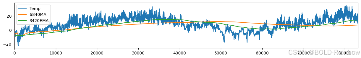
查看我们的数据,我们可以看到温度测量存在明显的季节性趋势,此时,我们可能有兴趣了解数据中的哪些因素导致了这种温度趋势。这个概念称为因果关系,将在本书的后面一章中讨论。
动量策略
动量用来衡量当前或未来趋势的强度,而不论其方向,即是上升还是下降。 它纯粹是一种技术分析技巧,并不考虑公司的基本面。 交易者在趋势强劲或价格行动动量大的情况下使用短期动量策略。 高动量指标是指价格在短时间内大范围上涨或下跌。 高动量也表明波动性增加。
动量投资者试图理解和预测市场行为,因为对其他投资者的偏见和情绪的认识能让动量投资策略更好地发挥作用。
如何运用动量策略
-
交易者使用趋势线、移动平均线和 ADX 等指标检查趋势是否存在。
-
当趋势获得动量(增强)时,交易者决定跟随趋势方向采取何种仓位(买入上升趋势;卖出下降趋势)。
-
当趋势势头出现减弱迹象时,交易者就会退出。 价格走势与 MACD 或 RSI 等动量指标走势之间的背离是一种常见指标。
Example 6: Momentum Trading Strategy Using Two MA’s
如上所述,动量策略可以在使用移动平均线检查趋势后应用。 SMA 和 EMA 被广泛应用于股票价格的技术分析和买卖信号的生成。 其基本原理是使用两个不同的窗口(短观察窗口和长观察窗口),并观察两条移动平均线的交叉点。 与长窗口相比,短窗口对价格变化的反应更快。 因此,如果 M A ( n = s h o r t ) > M A ( n = l o n g ) \mathrm{MA(n=short)>MA(n=long)} MA(n=short)>MA(n=long),交易策略或信号就是买入。 否则,信号就是卖出。
均线在技术分析中运行良好,但它的行为滞后于当前价格的 𝑛 / 2 𝑛/2 n/2 天。 这意味着只有在滞后几天后才能看到趋势的变化,从而导致策略延迟。 由于权重是以指数形式递减的,因此 EMA 大大减少了这种滞后性。 我们始终采用相同的策略,即在观察窗口较短和较长的两个 EMA 之间寻找交叉点,也就是说,当观察窗口较短的 EMA 穿过观察窗口较长的 EMA 时,就会产生买入信号。
现在,让我们用 Netflix 的数据来演示如何使用 MA 和 EMA 来发出信号或决定买入或卖出股票。
# Recall Netflix data we used above in forecasting using linear regression (LR)
plt.rcParams["figure.figsize"] = (15,2)
price.plot()
plt.ylabel('Price')
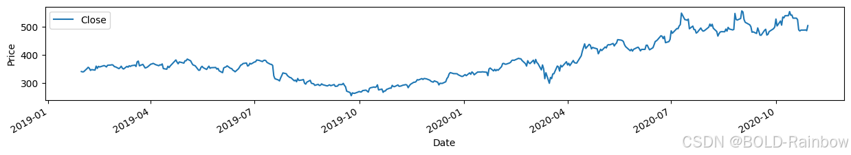
我们将对短期 MA 使用 n = 25 n=25 n=25 的窗口大小,对长期 MA 使用 n = 65 n=65 n=65 的窗口大小。
## In pandas, the rolling windows is available in computing for the mean of a window sized-n.
price['20MA'] = price['Close'].rolling(window=20, min_periods=1).mean()
price['65MA'] = price['Close'].rolling(window=65, min_periods=1).mean()
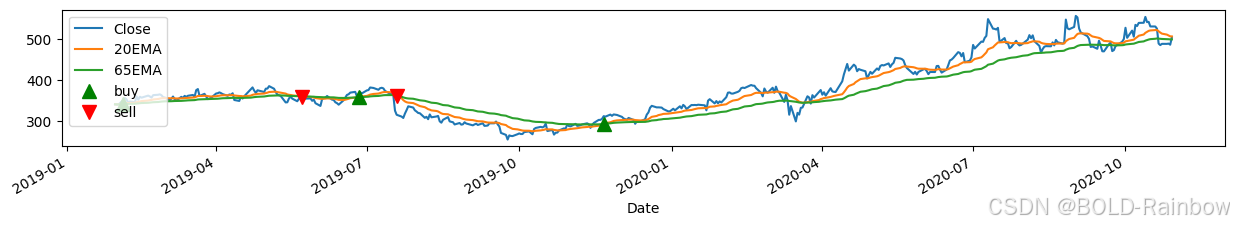
我们将尝试找到两条 MA 的交叉点,并创建一个交叉 “指标”。 请注意,该指标与上文讨论的指标 "I "并不完全相同。 然后,我们将根据生成的指标创建策略。 该策略基于价格走势。
如果 MA20> MA65,则指标等于+1.0,否则指标等于 0.0。 一旦出现交叉,MA20 和 MA65 的位置就会反转。 因此,得到指标 ( I d i f f = I t − I t − 1 ) (I_{diff}=I_t-It-1) (Idiff=It−It−1)之间的差值 连续两次,我们就能知道反转是正值(买入)还是负值(卖出)。
price['Indicator'] = 0.0
price['Indicator'] = np.where(price['20MA']> price['65MA'], 1.0, 0.0)

# To get the difference of the indicators, we use function diff in pandas.
price['Decision'] = price['Indicator'].diff()
# print(price)
#Decision=+1 means buy, while Decision=-1 means sell
# plotting them all together
price['Close'].plot(label= 'Close')
price['20MA'].plot(label = '20MA')
price['65MA'].plot(label = '65MA')

plt.plot(price[price['Decision'] == 1].index, price['20MA'][price['Decision'] == 1], '^', markersize = 10, color = 'g' , label = 'buy')
plt.plot(price[price['Decision'] == -1].index, price['20MA'][price['Decision'] == -1],  'v', markersize = 10, color = 'r' , label = 'sell')
plt.legend(loc='upper left')

使用两个 MA 并获取它们的交叉或差异作为指标,我们可以决定是买入(绿色)股票还是卖出(红色)。我们可以使用 EMA 执行与上面相同的过程。
# In pandas, the rolling window equivalent for EMA is
price['20EMA'] = price['Close'].ewm(span=20, adjust=False).mean()
price['65EMA'] = price['Close'].ewm(span=65, adjust=False).mean()
# Like how we used MA above, we will try to locate the crossover of the two EMAs and create an indicator of crossover
price['Indicator_EMA'] = 0.0
price['Indicator_EMA'] = np.where(price['20EMA']> price['65EMA'], 1.0, 0.0)

price['Decision_EMA'] = price['Indicator_EMA'].diff()
# print(price)
# Decision=+1 means buy, while Decision=-1 means sell
# plotting them all together
plt.rcParams["figure.figsize"] = (15,2)
price['Close'].plot(label= 'Close')
price['20EMA'].plot(label = '20EMA')
price['65EMA'].plot(label = '65EMA')

plt.plot(price[price['Decision_EMA'] == 1].index, price['20EMA'][price['Decision_EMA'] == 1], '^', markersize = 10, color = 'g' , label = 'buy')
plt.plot(price[price['Decision_EMA'] == -1].index, price['20EMA'][price['Decision_EMA'] == -1],  'v', markersize = 10, color = 'r' , label = 'sell')
plt.legend(loc='upper left')
对于这种情况,动量指标通常可以帮助我们做出是否买入的决定。交叉是趋势反转的迹象。在技术分析的背景下,“To buy” 预测价格会上涨,而 “To Sell” 预测价格会下跌。
这些工具通常有效,但还有更复杂的工具可用于进行技术分析。
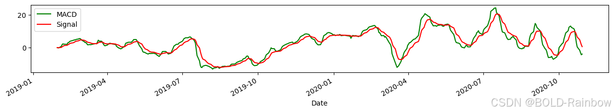
Example 7: Momentum Trading Strategy Using MACD
有许多动量交易策略可以使用。 在本例中,我们将使用Moving Average Convergence Divergence (MACD). MACD 是最流行的动量指标之一,它利用两条指数移动平均线(12 天和 26 天)之间的差值,并将其与 MACD 的 EMA(9 天)进行比较。
MACD Indicators
-
看涨交叉(买入)- MACD 在信号线上方交叉时出现。
-
看跌信号(卖出)–MACD 在信号线下方交叉。
-
超买或超卖 - 根据交叉是看涨还是看跌,交叉时 MACD 呈高斜率。 很快就会出现修正或方向反转。
-
运动中 - MACD 的小斜率显示运动较弱,修正的可能性很大,而运动较强,继续的可能性很大。
price['exp1'] = price['Close'].ewm(span=12, adjust=False).mean()
price['exp2'] = price['Close'].ewm(span=26, adjust=False).mean()
price['macd'] = price['exp1']-price['exp2']
price['exp3'] = price['macd'].ewm(span=9, adjust=False).mean()

price['macd'].plot(color = 'g', label = 'MACD')
price['exp3'].plot(color = 'r', label = 'Signal')
plt.legend(loc='upper left')

plt.show()
# Like how we used MA above, we will try to locate the crossover of the MACD and the Signal and plot the indicators
price['Indicator_MACD'] = 0.0
price['Indicator_MACD'] = np.where(price['macd']> price['exp3'], 1.0, 0.0)

price['Decision_MACD'] = price['Indicator_MACD'].diff()
# print(price)
price['macd'].plot(color = 'g', label = 'MACD')
price['exp3'].plot(color = 'r', label = 'Signal')
plt.legend(loc='upper left')

plt.plot(price[price['Decision_MACD'] == 1].index, price['macd'][price['Decision_MACD'] == 1], '^', markersize = 10, color = 'g' , label = 'buy')
plt.plot(price[price['Decision_MACD'] == -1].index, price['macd'][price['Decision_MACD'] == -1],  'v', markersize = 10, color = 'r' , label = 'sell')
plt.legend(loc='upper left')
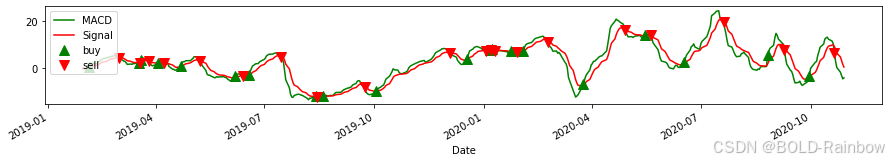
在上图中,我们可以看到看涨(买入)和看跌(卖出)交叉发生的大致日期。现在我们想要检查强度并确定超买和超卖情况。在这里,我们使用相同的参数,但我们绘制原始价格及其 MACD。
price['Close'].plot(color = 'k', label= 'Close')
price['macd'].plot(color = 'g', label = 'MACD')
plt.show()
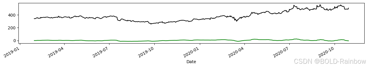
在这里,MACD 在某种程度上保持平坦,但请注意,有时 MACD 曲线比其他时间更陡峭,表明超买或超卖情况(例如 2020-04 年之前)。放大 MACD 图以查看斜率,我们有 ff:
fig, axs = plt.subplots(2, figsize=(15, 4), sharex=True)
axs[0].set_title('Close Price')
axs[1].set_title('MACD')
axs[0].plot(price['Close'], label='Close')
axs[1].plot(price['macd'], label='macd')
axs[1].set(xlabel='Date')
plt.show()
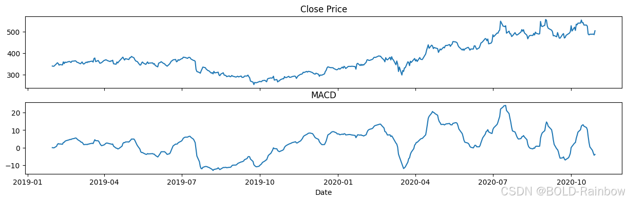
从上图可以看出,MACD 的陡峭斜率发生在 2020-04 年(超卖)和 2020-10 年(超买)之前。请注意,在 2020-07 年之后,MACD 仍有一些陡峭的斜率,这可能表明其他超买和超卖的情况。
最后,如上所述,交易中还使用了其他动量指标,例如 RSI 和 ADX。读者可以按照本笔记本中介绍的程序来探索它们。
Summary
在本章中,我们讨论并演示了如何使用线性、趋势和动量等预测工具。与上一章相比,我们注意到这里不需要检查时间序列的平稳性,也不需要进行差分。我们还展示了线性回归(以及多变量线性回归)在应用于某些数据时是有限的,并且表现不佳。最后,我们强调了虽然其他预测工具需要去除趋势,但在本笔记本中我们展示了可以利用趋势来预测数据的未来方向。


 2180
2180

 被折叠的 条评论
为什么被折叠?
被折叠的 条评论
为什么被折叠?
 到【灌水乐园】发言


