算法工程师17——典型代码

0 基本机器学习案例

0 目的
1 数据
2 数据探索
3 预处理
4 特征工程
5 数据打乱
6 数据集划分交叉验证
7 训练
8 划分不同的阈值和各种评价指标
8 预测
9 优化
10 保存

1 输入输出（输出字典的键和值）

# 1 读取一行
sys.stdin.readline()  
# 2 读取剩下所有行，这个有时候会出错
sys.stdin.readlines()
# 3 读取一行，以回车键为标记
 a = input()
 b, c = a.split(' ')
# 4 strip删去首尾指定字符串https://www.runoob.com/python/att-string-strip.html
# 不放参数默认删除空格和换行符
注意：该方法只能删除开头或是结尾的字符或字符串，不能删除中间部分的字符。
str = "00000003210Runoob01230000000"; 
print str.strip( '0' );  # 去除首尾字符 0
# 5 安指定字符分割.split()，默认以空格和\n，或\n
str = "Line1-abcdef \nLine2-abc \nLine4-abcd";
print str.split( );       # 以空格为分隔符，包含 \n
print str.split(' ', 1 ); # 以空格为分隔符，分隔成两个
输出
['Line1-abcdef', 'Line2-abc', 'Line4-abcd']
['Line1-abcdef', '\nLine2-abc \nLine4-abcd']
# 6 将一行输入分割并转换为数字类型
for _ in range(n):
    a,b = map(int,input().strip().split())
    print(a+b)
# 7 遍历字典
kkk = {"lx":25,"dy":"gril"}
for i,v in kkk.items():
    print(i,v)
输出：
lx 25
dy gril

2 numpy和cv实现影像平滑和显示

import numpy as np
print(np.random.rand(5,5)) #产生2行三列均匀分布随机数组
print(np.random.randn(5,5))# 正态分布随机数据
print(np.random.randint(1,10,[5,5]))   #(1,100）以内的5行5列随机整数
print(np.random.random(25).reshape(5,5))  #(0,1）以内10个随机浮点数
index = np.random.choice(np.arange(n), size=5, replace=False) # 随机选5个不重复的
np.random.seed(1234) #设置随机种子为1234
a=np.arange(10)
b=np.random.permutation(a) # 对数组进行打乱
np.random.shuffle(a)# 对数组进行打乱，原数组会改变
np.expand_dims(arr, axis) # 增加维度

print(a.dtype) # 获取类型
b= a.astype(np.uint8) # 转换类型
print(b.dtype)

image = cv2.imread(r'G:\baby.jpg')
image = cv2.cvtColor(image, cv2.COLOR_RGB2GRAY)
cv2.threshold(image, 140, 255, 0, image)
aa = cv2.resize(image,(400,200))
 
cv2.namedWindow("Image")
cv2.imshow("Image", aa)
cv2.waitKey(0)

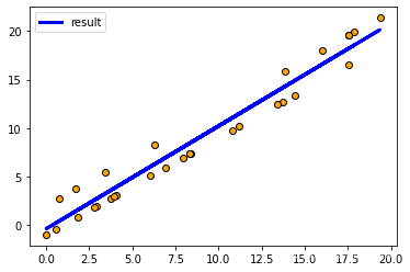
3 机器学习线性回归

# 生成数据
import matplotlib.pyplot as plt
#载入数据集
from sklearn.datasets import load_diabetes
#数据拆分工具
from sklearn.model_selection import train_test_split
# 数据拆分
from sklearn.model_selection import StratifiedKFold
# 线性回归
from sklearn.linear_model import LinearRegression
# 评分标准
from sklearn.metrics import f1_score
# 机器学习库
import lightgbm as lgb
# auc评判
from sklearn.metrics import roc_auc_score
# 均方根误差
from sklearn.metrics import mean_squared_error, r2_score
import numpy as np

# 1 数据
np.random.seed(1)
x1 = np.random.random(20)*20
y1 = x1-1
x2 = np.random.random(10)*20
y2 = x2+2
x = np.concatenate((x1,x2))
y = np.concatenate((y1,y2))
x = x.reshape(-1,1)
y = y.reshape(-1,1)

# 2 拆分成训练集和测试集
X_train,X_test,Y_train,Y_test=train_test_split(x,y,test_size=0.2,random_state=8)

# 3 回归问题能用交叉验证，但不能用StratifiedKFold

model = LinearRegression()   #实例化模型
model.fit(X_train, Y_train)  #用训练数据训练
# 系数的值
print('Coefficients: \n', model.coef_)
print(model.intercept_)
# 均方误差
y_train_predict = model.predict(X_train)
print('TRAIN_Mean squared error: %.2f' % mean_squared_error(Y_train, y_train_predict))
# r2决定系数: 1是完美预测,模型效果越好越接近1,效果越差越接近0
print('Coefficient of determinatino: %.2f' % r2_score(Y_train, y_train_predict))

y_pre = model.predict(X_test)
print('TEST_Mean squared error: %.2f' % mean_squared_error(Y_test, y_pre))

# 4 保存
import pickle #pickle模块

#保存Model(注:save文件夹要预先建立，否则会报错)
with open('Linear.pickle', 'wb') as f:
    pickle.dump(model, f)

#读取Model
with open('./Linear.pickle', 'rb') as f:
    model2 = pickle.load(f)
    #测试读取后的Model
    print(model2.predict([[2]]))

# 5 绘图
y_all_pre = model.predict(x)
plt.scatter(x,y,c="orange",edgecolors='k')  # 散点图
plt.plot(x, y_all_pre, color = 'blue', linewidth = 3,label="result")

plt.xticks()
plt.yticks()
plt.legend()
plt.show()

[1] (38条消息) Sklearn——用Sklearn实现线性回归(LinearRegression)_程旭员的博客-CSDN博客_sklearn实现线性回归
https://blog.csdn.net/weixin_37763870/article/details/105161775

4 机器学习xgb等

from sklearn.ensemble import RandomForestClassifier
from sklearn.metrics import accuracy_score
import lightgbm as lgb
import matplotlib.pyplot as plt
#载入数据集
from sklearn.datasets import load_diabetes
#数据拆分工具
from sklearn.model_selection import train_test_split
# 数据拆分
from sklearn.model_selection import StratifiedKFold
# 线性回归
from sklearn.linear_model import LinearRegression
# 评分标准
from sklearn.metrics import f1_score
# 机器学习库
import lightgbm as lgb
# auc评判
from sklearn.metrics import roc_auc_score
# 均方根误差
from sklearn.metrics import mean_squared_error, r2_score
import numpy as np

# 1 数据
np.random.seed(1)
x1 = np.random.random(20)*2
y1 = np.ones(20)
print(y1)
x2 = np.random.random(10)+5
y2 = np.zeros(10)
x = np.concatenate((x1,x2))
y = np.concatenate((y1,y2))
x = x.reshape(-1,1)
y = y.reshape(-1,1)
y.astype(np.int8)
for i,j in zip(x,y):
    print(i,j)

# 2 拆分成训练集和测试集
X_train,X_test,Y_train,Y_test=train_test_split(x,y,test_size=0.2,random_state=8)

# 3 五折交叉验证

N = 5
skf = StratifiedKFold(n_splits=N,shuffle=True,random_state=42)
for train_in,valid_in in skf.split(X_train,Y_train):
    # 构造训练集和验证集
    x_train,x_valid,y_tain,y_valid = X_train[train_in],X_train[valid_in],Y_train[train_in],Y_train[valid_in]
    
    # 下面是随机森林模型
    rfc = RandomForestClassifier(n_estimators=1000, max_depth=5, verbose=1)
    rfc.fit(x_train, y_tain)
    # f1得分
    y_valid_pred = rfc.predict(x_valid)
    print("准确率：",accuracy_score(y_valid, y_valid_pred))
    print("f1",f1_score(y_valid, y_valid_pred))
    print("roc",roc_auc_score(y_valid, y_valid_pred))
    

y_pre = rfc.predict(X_test)
print('TEST: %.2f' % f1_score(Y_test, y_pre))

### 下面是lgb模型
    # 创建lightGBM 输入数据，以及验证集
    lgb_train = lgb.Dataset(x_train, y_tain)
    lgb_eval = lgb.Dataset(x_valid, y_valid, reference=lgb_train)

    # lgm输入参数
    params = {
        'boosting_type': 'gbdt',
        'objective': 'binary',
        'metric': {'auc'},
        'num_leaves': 30,
        'learning_rate': 0.01,
        'feature_fraction': 0.7,
        'bagging_fraction': 0.8,
        'bagging_freq': 4,
        'verbose': 0,
        'lambda_l2':0.5,
        'lambda_l1':0.2
    }
    params['is_unbalance']='false'
    params['max_bin'] = 100
    params['min_data_in_leaf'] = 200
    print('Start training...')
    # 训练模型，这里使用的是lgm,提升树
    gbm = lgb.train(params,
                    lgb_train,
                    num_boost_round=20000,
                    valid_sets=lgb_eval,
                    verbose_eval=500,
                    early_stopping_rounds=50)

    print('Start predicting...')
    y_pred = gbm.predict(x_valid, num_iteration=gbm.best_iteration)
    print("lgb:",roc_auc_score(y_valid,y_pred))

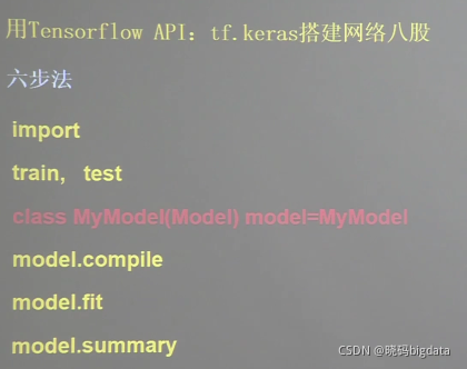
5 3层神经网络模型

import tensorflow as tf


mnist = tf.keras.datasets.mnist
(x_train, y_train), (x_test, y_test) = mnist.load_data()
x_train, x_test = x_train / 255.0, x_test / 255.0

model = tf.keras.models.Sequential([
    tf.keras.layers.Flatten(),
    tf.keras.layers.Dense(128, activation=tf.keras.activations.relu),
    tf.keras.layers.Dense(10, activation=tf.keras.activations.softmax)
])

model.compile(optimizer=tf.keras.optimizers.Adam(),
              loss=tf.keras.losses.SparseCategoricalCrossentropy(from_logits=False),
              metrics=[tf.keras.metrics.sparse_categorical_accuracy])

model.fit(x_train, y_train, batch_size=32, epochs=5, validation_data=(x_test, y_test), validation_freq=1)
model.summary()

import tensorflow as tf


mnist = tf.keras.datasets.mnist
(x_train, y_train), (x_test, y_test) = mnist.load_data()
x_train, x_test = x_train / 255.0, x_test / 255.0
print(x_train.shape)


class MnistModel(tf.keras.Model):
    def __init__(self):
        super(MnistModel, self).__init__()
        self.flatten = tf.keras.layers.Flatten()
        self.d1 = tf.keras.layers.Dense(128, activation=tf.keras.activations.relu)
        self.d2 = tf.keras.layers.Dense(10, activation=tf.keras.activations.softmax)

    def call(self, inputs, training=None, mask=None):
        x = self.flatten(inputs)
        x = self.d1(x)
        y = self.d2(x)
        return y


model = MnistModel()

model.compile(optimizer=tf.keras.optimizers.Adam(),
              loss=tf.keras.losses.SparseCategoricalCrossentropy(from_logits=False),
              metrics=[tf.keras.metrics.sparse_categorical_accuracy])

model.fit(x_train, y_train, batch_size=32, epochs=5, validation_data=(x_test, y_test), validation_freq=1)
model.summary()

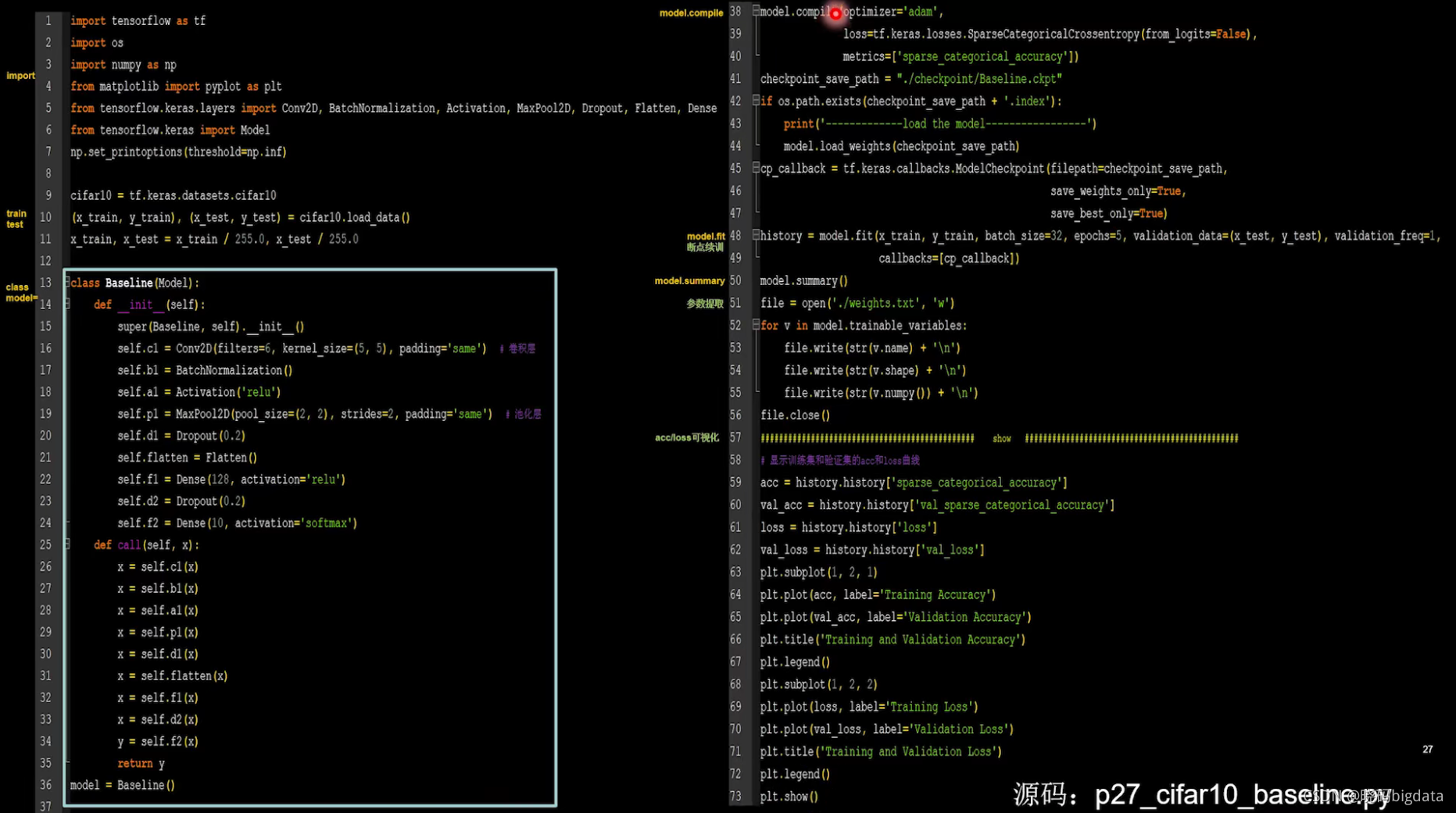
6 MobileNet

(38条消息) 神经网络学习小记录23——MobileNet模型的复现详解_Bubbliiiing的学习小课堂-CSDN博客
https://blog.csdn.net/weixin_44791964/article/details/102819915

7 Unet

# 实现了unet模型
import tensorflow as tf
import numpy as np


#########################################    2 前向传播
class Downsample(tf.keras.layers.Layer):
    "先定义，再调用,进行下采样"
    def __init__(self, units):
        "units是卷积核的数量"
        super(Downsample,self).__init__()
        # 使用了same填充，原论文使用valid填充
        self.conv1 = tf.keras.layers.Conv2D(units, kernel_size=3,padding="same")
        self.conv2 = tf.keras.layers.Conv2D(units, kernel_size=3, padding="same")
        # tf.keras.layers.MaxPooling2D()和tf.keras.layers.MaxPool2D()区别是什么？
        self.pool = tf.keras.layers.MaxPooling2D()

    def call(self, x, is_pool = True):
        if is_pool:
            x = self.pool(x)
        x = self.conv1(x)
        x = tf.nn.relu(x)
        x = self.conv2(x)
        x = tf.nn.relu(x)
        return x


class Upsample(tf.keras.layers.Layer):
    "先定义，再调用,进行上采样"
    def __init__(self, units):
        "units是卷积核的数量"
        super(Upsample, self).__init__()
        self.conv1 = tf.keras.layers.Conv2D(units, kernel_size=3, padding="same")
        self.conv2 = tf.keras.layers.Conv2D(units, kernel_size=3, padding="same")
        self.deconv = tf.keras.layers.Conv2DTranspose(units//2,kernel_size=3,strides=2,padding="same")

    def call(self, x):
        x = self.conv1(x)
        x = tf.nn.relu(x)
        x = self.conv2(x)
        x = tf.nn.relu(x)
        x = self.deconv(x)
        x = tf.nn.relu(x)
        return x

class Unet_model(tf.keras.Model):
    def __init__(self):
        "只进行初始化,定义层，还没有进行前向传播"
        super(Unet_model, self).__init__()
        # 这步只是进行卷积
        self.down1 = Downsample(64)

        # 4次下采样
        self.down2 = Downsample(128)
        self.down3 = Downsample(256)
        self.down4 = Downsample(512)
        self.down5 = Downsample(1024)

        # 4次上采样，定义一个上采样层
        # 第一个上采样只进行上采样，不进行卷积
        self.up1 = tf.keras.layers.Conv2DTranspose(512, kernel_size=3, strides=2, padding="same")
        # 上采样加卷积
        self.up2 = Upsample(512)
        self.up3 = Upsample(256)
        self.up4 = Upsample(128)

        # 进行两次卷积
        self.conv_last = Downsample(64)

        # 进行最后的1*1卷积分类，进行城市街景共34个类别的分类，所以输出层为34，，
        # 如果进行别的任务，是几类就写几，因为需要喝MeanIou一样，否则会报错
        self.last = tf.keras.layers.Conv2D(2, kernel_size=1, padding="same")

    def call(self, x):
        "进行前向传播模型的构建"

        # 第一次先进行两次卷积
        x1 = self.down1(x, is_pool = False)

        # 进行4次下采样加两次卷积
        x2 = self.down2(x1)
        x3 = self.down3(x2)
        x4 = self.down4(x3)
        x5 = self.down5(x4)

        # 进行一次上采样
        x5 = self.up1(x5)

        # 进行合并,然后卷积卷积上采样
        x6 = tf.concat([x4, x5], axis=-1)
        x6 = self.up2(x6)

        x7 = tf.concat([x3, x6], axis=-1)
        x7 = self.up3(x7)

        x8 = tf.concat([x2, x7], axis=-1)
        x8 = self.up4(x8)

        # 合并，然后两层卷积
        x9 = tf.concat([x1, x8], axis=-1)
        x9 = self.conv_last(x9, is_pool = False)

        # 输出为34层，共34个类别
        out = self.last(x9)

        return out

train_history = model.fit(
    data_train,
    epochs=50,
    steps_per_epoch=train_count // BATCH_SIZE,
    validation_data=data_test,
    validation_freq=1,
)

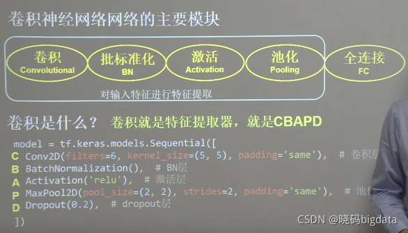
8 卷积就是CM

(38条消息) 图像分类网络6——VGG16识别5分类（ImageDataGenerator和迁移学习）_xiaotiig的博客-CSDN博客
https://blog.csdn.net/xiaotiig/article/details/115699491

9 tf的常用接口

[1] (38条消息) TensorFlow的 各模块关系keras、nn、metrics、model、Sequential、data.Dataset、keras.datasets_尚墨1111的博客-CSDN博客
https://blog.csdn.net/qq_42647903/article/details/109095372?spm=1001.2101.3001.6650.1&utm_medium=distribute.pc_relevant.none-task-blog-2%7Edefault%7ECTRLIST%7Edefault-1.no_search_link&depth_1-utm_source=distribute.pc_relevant.none-task-blog-2%7Edefault%7ECTRLIST%7Edefault-1.no_search_link

[2] Module: tf | TensorFlow Core v2.6.0
https://tensorflow.google.cn/api_docs/python/tf

[3] 【北京大学】Tensorflow2.0_哔哩哔哩_bilibili
https://www.bilibili.com/video/BV1B7411L7Qt?from=search&seid=10450977565826079889&spm_id_from=333.337.0.0

10 gdal的几个接口

[1] Python地理空间数据处理、分析与可视化_哔哩哔哩_bilibili
https://www.bilibili.com/video/BV1Fy4y1y7U6?spm_id_from=333.999.0.0
[2] GDAL书