使用TensorFlow编程实现一元逻辑回归

xuechanba

已于 2022-05-07 19:17:21 修改

阅读量1.7k

点赞数

文章标签： tensorflow 逻辑回归 python

于 2022-05-02 14:43:18 首次发布

本文链接：https://blog.csdn.net/xuechanba/article/details/124530357

版权

内容回顾

逻辑回归是在线性模型的基础上，再增加一个Sigmoid函数来实现的。
在这里插入图片描述
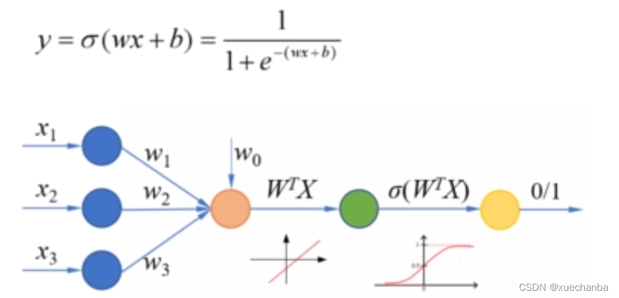
输入样本特征，经过线性组合之后，得到的是一个连续值，经过Sigmoid函数，把它转化为一个0-1之间的概率，再通过设置一个合理的阈值，就可以实现二分类问题。

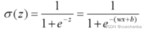
Sigmoid 函数：

在实现逻辑回归时，需要计算
在这里插入图片描述
如何编程来实现这个函数表达式：

import numpy as np
import tensorflow as tf

# 在TensorFlow中, 使用 exp 来实现 e^x 的运算,
# 需要注意这个函数的参数要求是浮点数。
x = np.array([1., 2., 3., 4.])

w = tf.Variable(1.)
b = tf.Variable(1.)

print(1/(1+tf.exp(-(w*x+b))))
"""
tf.Tensor([0.880797   0.95257413 0.98201376 0.9933072 ], shape=(4,), dtype=float32)
"""

准确率：

在这里插入图片描述

import numpy as np
import tensorflow as tf

# 假设 y 是样本标签
y = np.array([0, 0, 1, 1])
# pred 是对应的预测概率
pred = np.array([0.1, 0.2, 0.8, 0.49])

# 如果将阈值设置为 0.5 ,就可以使用四舍五入函数 round, 把它转换为 0 和 1
print(tf.round(pred))
"""
tf.Tensor([0. 0. 1. 0.], shape=(4,), dtype=float64)
"""

# 然后使用 equal 函数逐个元素的去比较预测值和标签值
print(tf.equal(tf.round(pred), y))
"""
tf.Tensor([ True  True  True False], shape=(4,), dtype=bool)
"""

# 使用 cast 函数将上面得到的结果转换为整数
print(tf.cast(tf.equal(tf.round(pred), y), tf.int8))
"""
tf.Tensor([1 1 1 0], shape=(4,), dtype=int8)
"""

# 得到预测正确的样本数在所有样本数中的比例
print(tf.reduce_mean(tf.cast(tf.equal(tf.round(pred), y), tf.float32)))
"""
tf.Tensor(0.75, shape=(), dtype=float32)
"""

# 需要注意的是, 使用 round 函数时, 如果参数恰好是0.5, 那么返回的结果是0.0
print(tf.round(0.5))
"""
tf.Tensor(0.0, shape=(), dtype=float32)
"""

# 当参数的值大于0.5时, 返回的结果才是是1.0
print(tf.round(0.5000001))
"""
tf.Tensor(1.0, shape=(), dtype=float32)
"""

在上面例子中，阈值被设置为0.5，如果想要设置为其他值，应该怎么处理呢？
可以使用 TensorFlow 中的 where 函数。

where (condition, a, b)
# 它根据condition返回a或者b的值，参数condition是一个布尔型的张量或者数组。
# 如果condition中的某个元素为真，那么对应位置就返回 a ，否则返回 b 。

例子如下：

import numpy as np
import tensorflow as tf

# pred 是预测概率
pred = np.array([0.1, 0.2, 0.8, 0.49])

print(pred < 0.5)
# [ True  True False  True]

print(tf.where(pred < 0.5, 0, 1))
# tf.Tensor([0 0 1 0], shape=(4,), dtype=int32)

print(pred < 0.4)
# [ True  True False False]

print(tf.where(pred < 0.4, 0, 1))
# tf.Tensor([0 0 1 1], shape=(4,), dtype=int32)

参数 a 和 b还可以是张量或者数组，这时a和b必须有相同的形状。并且它们的第一维必须和condition形状一致。

import numpy as np
import tensorflow as tf

# pred 是预测概率
pred = np.array([0.1, 0.2, 0.8, 0.59])

a = np.array([1, 2, 3, 4])
b = np.array([10, 20, 30, 40])

print(tf.where(pred < 0.5, a, b))
# tf.Tensor([ 1  2 30  40], shape=(4,), dtype=int32)

print(tf.where(pred >= 0.5))
# 当参数 a 和 b 省略时, 就返回数组 pred 中大小等于0.5的元素的索引
# 这个返回值以一个二维张量的形式给出
"""
tf.Tensor(
[[2]
 [3]], shape=(2, 1), dtype=int64)
"""
# 这在我们需要获取某种条件的掩码时非常有用

# 在计算分类准确率时, 使用 where 函数可以更加灵活地设置阈值
# 然后将预测概率转化为类别
y = np.array([0, 0, 1, 1])
y_pred = np.array([0.1, 0.2, 0.8, 0.49])

print(tf.reduce_mean(tf.cast(tf.equal(tf.where(y_pred < 0.5, 0, 1), y), tf.float32)))
"""
tf.Tensor(0.75, shape=(), dtype=float32)
"""

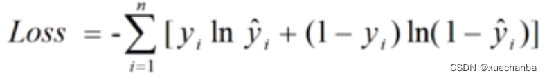
交差熵损失函数：

在这里插入图片描述

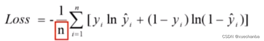
平均交差熵损失函数：

在这里插入图片描述

import numpy as np
import tensorflow as tf

# 假设 y 是样本标签
y = np.array([0, 0, 1, 1])
# pred 是对应的预测概率
pred = np.array([0.1, 0.2, 0.8, 0.49])

# 计算交差熵损失函数值
# tf.math.log实现以 e 为底的对数运算
print(-tf.reduce_sum(y*tf.math.log(pred)+(1-y)*tf.math.log(1-pred)))
# tf.Tensor(1.2649975061637104, shape=(), dtype=float64)

# 计算平均交差熵损失函数值
print(-tf.reduce_mean(y*tf.math.log(pred)+(1-y)*tf.math.log(1-pred)))
# tf.Tensor(0.3162493765409276, shape=(), dtype=float64)

实例：实现一元逻辑回归
在这里插入图片描述
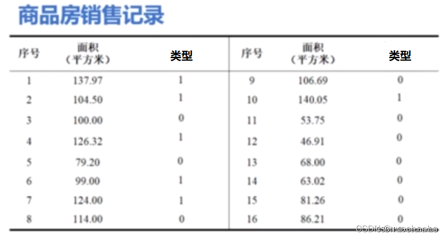
（这个图中的数据比前面的不一样，修改了两个数据，目的是为了和其他相邻的点重合。其中，0代表普通住宅，1代表高档住宅。）

注意，在训练模型时，是没有房价这个标签的，而是直接使用面积和所属的类别来训练模型。

此外，在模型的训练过程中产生的线性模型 wx + b 的值，我们可以把它理解为类似于房价的一个指标，它是一个中间结果，我们并不需要把它读取出来。

第一步：加载数据

代码如下：

import numpy as np
import tensorflow as tf

import matplotlib.pyplot as plt

plt.rcParams["font.family"] = "SimHei", "sans-serif"
plt.rcParams['axes.unicode_minus'] = False  # 设置正常显示符号

# 第一步：数据加载

# 面积都是大于40的正数
x = np.array([137.97, 104.50, 100.00, 126.32, 79.20, 99.00, 124.00, 114.00,
              106.69, 140.05, 53.75, 46.91, 68.00, 63.02, 81.26, 86.21])

y = np.array([1, 1, 0, 1, 0, 1, 1, 0, 0, 1, 0, 0, 0, 0, 0, 0])

plt.figure()
plt.scatter(x, y)
plt.show()

运行下代码：
在这里插入图片描述
（注：面积都是大于40的正数）

第二步：数据处理

因为 Sigmoid 函数是以零点为中心的，因此在数据处理阶段, 我们对这些点进行中心化，每个样本点都减去它们的平均值，这样整个数据集的均值就等于0。

x_train = x - np.mean(x)
y_train = y


plt.figure()
plt.scatter(x_train, y_train)
plt.suptitle("数据处理后的商品房分类图", fontsize=20)
plt.show()

在运行下代码：
在这里插入图片描述
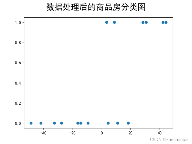
可以发现，数据整体向左平移了，但是它们之间的想对位置并没有改变。

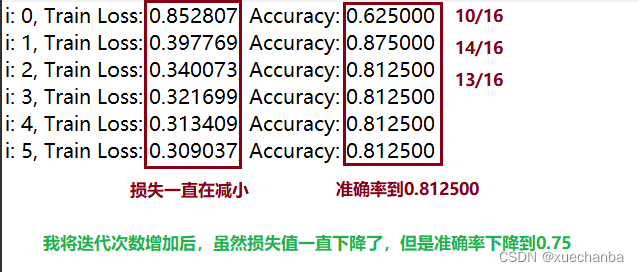
第三步：设置超参数

learn_rate = 0.005
itar = 5
display_step = 1

第四步：训练模型

cross_train = []  # 用来存放训练集的交叉熵损失
acc_train = []  # 用来存放训练集的分类准确率

for i in range(0, itar+1):

    with tf.GradientTape() as tape:

        # Sigmoid 函数
        pred_train = 1/(1+tf.exp(-(w*x_train+b)))
        # 平均交叉熵损失函数
        Loss_train = -tf.reduce_mean(y_train * tf.math.log(pred_train) + (1 - y_train) * tf.math.log(1 - pred_train))
        # 计算准确率函数 -- 因为不需要对其进行求导运算, 因此也可以把这条语句写在 with 语句的外面
        Accuarcy_train = tf.reduce_mean(tf.cast(tf.equal(tf.where(pred_train < 0.5, 0, 1), y_train), tf.float32))

    # 记录每一次迭代的交叉熵损失和准确率
    cross_train.append(Loss_train)
    acc_train.append(Accuarcy_train)

    # 对交叉熵损失函数分别对 w 和 b 求偏导
    dL_dw, dL_db = tape.gradient(Loss_train, [w, b])

    # 更新模型参数
    w.assign_sub(learn_rate * dL_dw)
    b.assign_sub(learn_rate * dL_db)

    if i % display_step == 0:
        print("i: %i, Train Loss: %f, Accuracy: %f" % (i, Loss_train, Accuarcy_train))

运行结果如下：
在这里插入图片描述

第六步：数据可视化

1、绘制 Sigmoid 函数曲线图

# 在设置模型初始值后, 给出一组连续的x坐标
x_ = range(-80, 80)
# 并使用 w 和 b 的初始值，计算Sigmoid 函数作为 y 坐标
y_ = 1/(1+tf.exp(-(w*x_+b)))

在这里插入图片描述
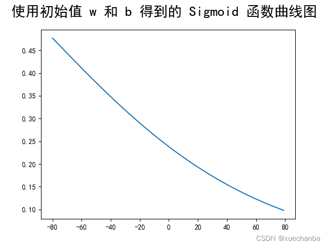
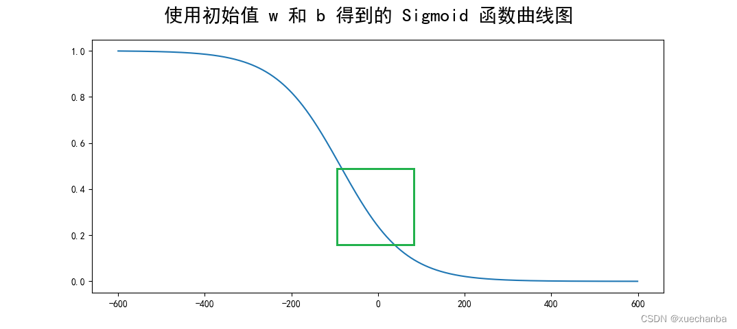
这个曲线看起来和S型曲线相差很大，是因为这个随机的w和b正好得到了一个中间变化部分范围很大的曲线。
如果将 x 取值扩大一些，比如扩大到

# 在设置模型初始值后, 给出一组连续的x坐标
x_ = range(-600, 600)
# 并使用 w 和 b 的初始值，计算Sigmoid 函数作为 y 坐标
y_ = 1/(1+tf.exp(-(w*x_+b)))

此时，再来看看输出图像
在这里插入图片描述
接下来，在训练模型的过程中增加绘制 Sigmoid 函数曲线图。

# 第四步：设置模型变量的初始值
......

# 在设置模型初始值后, 给出一组连续的x坐标
x_ = range(-80, 80)
# 并使用 w 和 b 的初始值，计算Sigmoid 函数作为 y 坐标
y_ = 1/(1+tf.exp(-(w*x_+b)))

plt.figure()
# 绘制房子实际分类的散点图
plt.scatter(x_train, y_train)
plt.plot(x_, y_, color="red", linewidth=3)

# 第五步：训练模型
......
for i in range(0, itar+1):

    with tf.GradientTape() as tape:
    ......
    ......
     if i % display_step == 0:
        print("i: %i, Train Loss: %f, Accuracy: %f" % (i, Loss_train, Accuarcy_train))
        y_ = 1/(1+tf.exp(-(w*x_+b)))
        plt.plot(x_, y_)

plt.suptitle("不断更新 w 和 b 后得到的 Sigmoid 函数曲线图", fontsize=20)
plt.show()

运行结果如下：
在这里插入图片描述
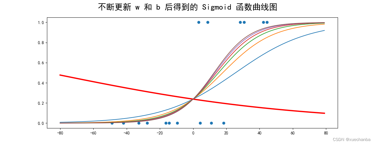
上图红色的粗线是随机设置模型参数 w 、b的初始值后绘制出来的曲线，可以看出刚好有10个点属于普通住宅，这只能说是运气蒙对了。

上图蓝色的（曲））线是第一次迭代后的结果，随着迭代次数增加，输出概率越来越能够反映出样本的真实分类了。

那怎么根据曲线来判断出分类的呢？
是根据每个样本点在曲线上对应的取值，再与0.5进行比较，低于0.5时，被分类为普通住房，而高于0.5时，则被分类为高档住宅。

因为下图框中的圈起来的这几个样本（横坐标为0附近）），该位置的曲线斜率较大，更新后的 w 和 b 对该曲线的斜率的影响也是最大的，比较难预测。
在这里插入图片描述
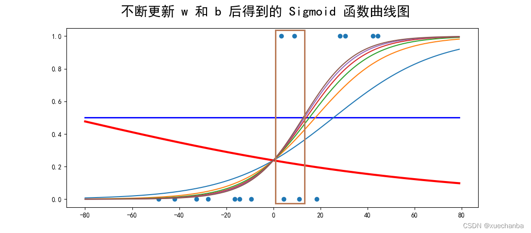
所以这个区域中的点可能会出现分类错误，导致准确率无法达到100%。

第一次训练的模型分类的准确率虽然更高，但是从整体上来看，还是经过更多次迭代之后概率的预测更加合理。

第七步：模型预测

# 第七步：模型预测

x_test = np.array([128.15, 45.00, 141.43, 106.27, 99.00, 53.84, 85.36, 70.00, 162.00, 114.60])

# 这里使用训练数据的平均值对新的数据进行中心化处理
pred_test = 1 / (1 + tf.exp(-(w * (x_test-np.mean(x)) + b)))

# 根据概率进行分类
y_test = tf.where(pred_test < 0.5, 0, 1)

for i in range(len(x_test)):
    print(x_test[i], "\t", pred_test[i].numpy(), "\t", y_test[i].numpy())

输出结果如下：

"""
128.15 	 0.8610252 	     1
45.0 	 0.0029561974 	 0
141.43 	 0.9545566 	     1
106.27 	 0.45318928 	 0
99.0 	 0.2981362 	     0
53.84 	 0.00663888 	 0
85.36 	 0.108105935 	 0
70.0 	 0.028681064 	 0
162.0 	 0.9928677 	     1
114.6 	 0.6406205 	     1
"""

要注意的是，这里虽然使用 x_test 来表示这些数据，但是它并不是测试集，因为真正的测试集是有标签的数据，例如波士顿房价数据集中的测试集。在训练的过程中，通过模型在测试集上表现来评价模型的性能。在机器学习中，要求测试集和训练集是独立同分布的。也就是说，它们有着相同的均值和方差。这样的测试才有意义。

而这里的 x_test，实际上是模型训练好之后，在真实场景下的应用情况，是没有标签的。真实场景中的数据，可能是各种各样的，而且通常来说，每次应用可能只是给出一个数据，或者一部分数据，所以这里采用训练集中的均值来中心化数据。

下面来将数据可视化。首先，根据分类结果绘制散点图，可以看到这四套商品房被划分为高档住宅，剩下的被划分为普通住宅。通过散点图，可以更加直观地得到商品房类型和面积的关系，然后绘制概率曲线。

plt.subplot(122)
plt.title("Test Outcome", fontsize=12)
plt.scatter(x_test, y_test)
x_ = np.array(range(-80, 80))
y_ = 1/(1 + tf.exp(-(w * x_ + b)))
plt.plot(x_+np.mean(x), y_)
plt.show()

运行结果如下：
在这里插入图片描述
因为散点图的 x 坐标使用的是真实的面积，没有平移，所以在这里加上训练集的均值。

xuechanba

关注

0
点赞
踩
7

收藏

觉得还不错? 一键收藏
打赏
0
评论
使用TensorFlow编程实现一元逻辑回归

在实现逻辑回归时，需要计算Sigmoid 函数：如何编程来实现这个函数表达式：import numpy as npimport tensorflow as tf# 在TensorFlow中, 使用 exp 来实现 e^x 的运算,# 需要注意这个函数的参数要求是浮点数。x = np.array([1., 2., 3., 4.])w = tf.Variable(1.)b = tf.Variable(1.)print(1/(1+tf.exp(-(w*x+b))))"""tf.Te
复制链接

扫一扫