线性回归与逻辑回归

$\frac{\partial J\left( \theta \right)}{\partial\theta} = \frac{1}{n}\sum_{i = 1}^{n}{\lbrack\left( \theta^{T}x_{i} - y_{i} \right)x_{\text{ij}}\rbrack} = \frac{1}{n}X^{T}(X\theta - Y)$

逻辑回归：使用sigmod/softmax作为联系函数，交叉熵作为损失函数。

二分类：使用sigmod作为联系函数

$\frac{1}{1 + e^{- z}}$

$J\left( \theta \right) = C_{0} = - \frac{1}{n}\sum_{i = 1}^{n}{\lbrack y_{i}\log\left( sigmod(\theta^{T}x_{i}) \right) + \left( 1 - y_{i} \right)\log{\left( 1 - {sigmod(\theta}^{T}x_{i} \right))}\rbrack}$

$\frac{\partial J\left( \theta \right)}{\partial\theta} = \frac{1}{n}\sum_{i = 1}^{n}{\lbrack\left( sigmod(\theta^{T}x_{i}) - y_{i} \right)x_{\text{ij}}\rbrack} = \frac{1}{n}X^{T}(sigmod(X\theta) - Y)$

多分类：使用softmax作为联系函数，y采用独热编码。

引入指数形式的缺点
指数函数的曲线斜率逐渐增大虽然能够将输出值拉开距离，但是也带来了缺点，当值非常大的话，计算得到的数值也会变的非常大，数值可能会溢出。

当然针对数值溢出有其对应的优化方法，将每一个输出值减去输出值中最大的值。

$\max_{1\leq j\leq m}{z},softmax = \frac{e^{z}}{\sum_{0 \leq j \leq m}^{}e^{z}}$

$J\left( \theta \right) = C_{0} = - \frac{1}{n}\sum_{i = 1}^{n}{y_{i}\log\left( softmax(\theta^{T}x_{i}) \right)}$

$\frac{\partial J\left( \theta \right)}{\partial\theta} = \frac{1}{n}\sum_{i = 1}^{n}{\lbrack\left( softmax(\theta^{T}x_{i}) - y_{i} \right)x_{\text{ij}}\rbrack} = \frac{1}{n}X^{T}(softmax(X\theta) - Y)$

3.1.2.1 梯度下降

随机梯度下降：

$\theta_{t + 1} = \theta_{t} - \alpha\nabla_{\theta}J(\theta_{t})$

$\theta_{t}$ 是在迭代步骤t的参数， $\alpha$ 是学习率， $J(\theta_{t})$ 是损失函数， $\nabla_{\theta}J(\theta_{t})$ 是损失函数关于参数 $\theta_{t}$ 的梯度。

批量梯度下降：

$\theta_{t + 1} = \theta_{t} - \alpha\nabla J_{i}(\theta_{t})$

$\theta_{t}$ 是在迭代步骤t的参数， $\alpha$ 是学习率， $J_{i}$ 是对第i个数据点计算的损失函数， $\nabla J_{i}(\theta_{t})$ 是在当前参数 $\theta_{t}$ 下的梯度。

3.1.2.2 公式法

$\theta = \left( X^{T}X \right)^{- 1}X^{T}\text{Y\ }$

3.1.3 特征缩放

使用Standardization，将数据变为均值为0，方差为1的正态分布。

$x^{'} = \frac{x - \mu}{\sigma}$

3.1.4 正则化

L1，L2正则化

L1正则化： $C_{0} + \frac{\lambda}{n}\sum_{\theta}^{}{|\theta|}$

$\frac{\partial C}{\partial\theta} = \frac{\partial C_{0}}{\partial\theta} + \frac{\lambda}{n}\theta$

L2正则化： $C_{0} + \frac{\lambda}{2n}\sum_{\theta}^{}\theta^{2}$

$\frac{\partial C}{\partial\theta} = \frac{\partial C_{0}}{\partial\theta} + \frac{\lambda}{n}sgn(\theta)$

3.1.5 可视化方法

使用matplolib，seaborn

3.1.6 模型评估

线性回归：

$\overline{y} = \frac{1}{n}\sum_{i = 1}^{n}y_{i}$

$\text{SS}_{\text{tot}} = \sum_{i = 1}^{n}\left( y_{i} - \overline{y} \right)^{2}$

$\text{SS}_{\text{reg}} = \sum_{i = 1}^{n}\left( {\widehat{y}}_{i} - \overline{y} \right)^{2}$

$\text{SS}_{\text{res}} = \sum_{i = 1}^{n}\left( y_{i} - {\widehat{y}}_{i} \right)^{2}$

$R^{2} = 1 - \frac{\text{SS}_{\text{res}}}{\text{SS}_{\text{tot}}}$

逻辑回归：

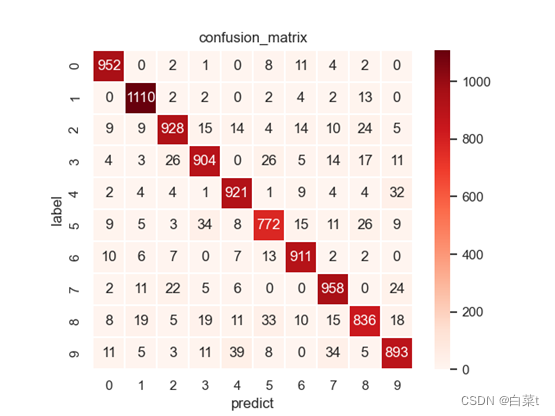
混淆矩阵：cm[i, j]表示真实标签为i预测标签为j的个数。(m, m)的形状。

TP：cm矩阵的对角线值

FP： $\sum_{i = 1}^{m}{cm\lbrack i,\ \ :\rbrack} - TP$ （cm列求和-TP）

FN： $\sum_{j = 1}^{m}{cm\lbrack:,\ \ j\rbrack} - TP$ （cm行求和-TP）

TN： $c\text{m.sum}() - TP - FP - FN$

P： $\frac{1}{m}\sum_{i = 1}^{m}\frac{\text{TP}}{TP + FP}$

R： $\frac{1}{m}\sum_{i = 1}^{m}\frac{\text{TP}}{TP + FN}$

A： $\frac{\text{TP}\text{.sum}()}{\ cm.sum()\ }$

F1： $\frac{2\text{PR}}{P + R}$

3.1.7 性能需求

无性能需求

3.2 系统结构图

3.3 关键技术难点的实现

3.3.1 线性回归模型构造

3.3.1.1线性回归

正向传播： $\widehat{y} = X\theta$

损失函数计算： $J\left( \theta \right) = C_{0} = \frac{1}{2n}\sum_{i = 1}^{n}\left( y_{i} - {\widehat{y}}_{i} \right)^{2}$

反向传递： $\frac{\partial J\left( \theta \right)}{\partial\theta} = \frac{1}{n}X^{T}(X\theta - Y)$ ,
$\theta = \theta - \alpha\frac{\partial J\left( \theta \right)}{\partial\theta}$

3.3.1.2逻辑回归

二分类：

正向传播： $\ \widehat{y} = sigmod(X\theta)$

L1正则化：

$J\left( \theta \right) = C_{0} = - \frac{1}{n}\sum_{i = 1}^{n}\left\lbrack y_{i}\log\left( {\widehat{y}}_{i} \right) + \left( 1 - y_{i} \right)\log\left( 1 - {\widehat{y}}_{i} \right) \right\rbrack + \frac{\lambda}{n}\sum_{\theta}^{}{|\theta|}$

$\frac{\partial J\left( \theta \right)}{\partial\theta} = \frac{1}{n}\sum_{i = 1}^{n}{\lbrack\left( {\widehat{y}}_{i} - y_{i} \right)x_{\text{ij}}\rbrack} + \frac{\lambda}{n}\text{sgn}\left( \theta \right) = \frac{1}{n}X^{T}\left( \widehat{y} - Y \right) + \frac{\lambda}{n}sgn(\theta),\ \theta = \theta - \alpha\frac{\partial J\left( \theta \right)}{\partial\theta}$

L2正则化：

$\frac{\partial J\left( \theta \right)}{\partial\theta} = \frac{1}{n}\sum_{i = 1}^{n}{\lbrack\left( {\widehat{y}}_{i} - y_{i} \right)x_{\text{ij}}\rbrack} + \frac{\lambda}{n}\theta = \frac{1}{n}X^{T}\left( \widehat{y} - Y \right) + \frac{\lambda}{n}\theta,\ \theta = \theta - \alpha\frac{\partial J\left( \theta \right)}{\partial\theta}$

多分类（y采用独热编码）：

正向传播： $\ \widehat{y} = \text{softmax}(X\theta)$

L1正则化：

$J\left( \theta \right) = C_{0} = - \frac{1}{n}\sum_{i = 1}^{n}{y_{i}\log\left( {\widehat{y}}_{i} \right)} + \frac{\lambda}{n}\sum_{\theta}^{}{|\theta|}$

L2正则化：

$J\left( \theta \right) = C_{0} = - \frac{1}{n}\sum_{i = 1}^{n}{y_{i}\log\left( {\widehat{y}}_{i} \right)} + \frac{\lambda}{2n}\sum_{\theta}^{}\theta^{2}$

$\frac{\partial J\left( \theta \right)}{\partial\theta} = \frac{1}{n}\sum_{i = 1}^{n}{\lbrack\left( {\widehat{y}}_{i} - y_{i} \right)x_{\text{ij}}\rbrack} + \frac{\lambda}{n}\theta = \frac{1}{n}X^{T}\left( \widehat{y} - Y \right) + \frac{\lambda}{n}\theta,\ \theta = \theta - \alpha\frac{\partial J\left( \theta \right)}{\partial\theta}$

3.3.2 TP、FP、TN及FN的取值

二分类：

TP：真实为真，预测为真；

FN：真实为真，预测为假；

FP：真实为假，预测为真；

TN：真实为假，预测为假；

多分类：

混淆矩阵：cm[i, j]表示真实标签为i预测标签为j的个数。(m, m)的形状。

TP：cm矩阵的对角线值

FP： $\sum_{i = 1}^{m}{cm\lbrack i,\ \ :\rbrack} - TP$ （cm列求和-TP）

FN： $\sum_{j = 1}^{m}{cm\lbrack:,\ \ j\rbrack} - TP$ （cm行求和-TP）

TN： $c\text{m.sum}() - TP - FP - FN$

3.3.4 混淆矩阵的求法

通过逻辑模型得到y的预测值，共有m类书，混淆矩阵cm设置为（m,
m）的形状，cm[i, j]=真实标签为i预测标签为j的个数。

直接求复杂度为 $O(\text{nm}^{2})$ ，在mnist数据集下计算很慢（n=10000），可以通过下面的方法快速求混淆矩阵，使用np.bincount方法计算每个类别组合的频次，需要将idx和label_y转换为一维数组，然后使用m
* label_y +
idx来获取每个元素的唯一索引，计算改数组中每个元素的频次，最后改变形状为（m,m）就能得到混淆矩阵。

也可以通过直接调用sklearn.metrics的confusion_matrix函数。cm =
confusion_matrix(label_y, idx, labels=[0, 1, 2, 3, 4, 5, 6, 7, 8, 9])

3.3.5 P、R、A、F1

二分类：

P = TP / (TP + FP)

A = (TP + TN) / (TP + FP + FN + TN)

R = TP / (TP + FN)

F1 = 2*P*R/(P+R)

多分类：

P： $\frac{1}{m}\sum_{i = 1}^{m}\frac{\text{TP}}{TP + FP}$

R： $\frac{1}{m}\sum_{i = 1}^{m}\frac{\text{TP}}{TP + FN}$

A： $\frac{\text{TP}\text{.sum}()}{\ cm.sum()\ }$

F1： $\frac{2\text{PR}}{P + R}$

3.3.6 三维平面和等高线的绘制

# 三维图和等高线
W = np.squeeze(W) #
原来是(n,1)的数组，必须转化为(n,)的数组，否则会报错
B = np.squeeze(B)

# Setup of meshgrid of theta values
T0, T1 = np.meshgrid(np.linspace(-1, 3, 100), np.linspace(-6, 2, 100))

# Computing the cost function for each theta combination
zs = np.array([cost(model(x, np.array([t0, t1]).reshape(-1, 1)),
y.reshape(-1, 1))
for t0, t1 in zip(np.ravel(T0), np.ravel(T1))])
# Reshaping the cost values
Z = zs.reshape(T0.shape)
anglesx = np.array(B)[1:] - np.array(B)[:-1]
anglesy = np.array(W)[1:] - np.array(W)[:-1]
ax = fig.add_subplot(2, 2, 3, projection=‘3d’)
ax.plot_surface(T0, T1, Z, rstride=5, cstride=5, cmap=‘jet’,
alpha=0.5)
ax.plot(B, W, costs, marker=‘*’, color=‘r’, alpha=.4, label=‘Gradient
descent’)

ax.set_xlabel(‘theta 0’)
ax.set_ylabel(‘theta 1’)
ax.set_zlabel(‘Cost function’)
ax.set_title(‘Gradient descent: Root at {}’.format(theta.ravel()))
ax.view_init(45, 45)

# Contour plot
ax = fig.add_subplot(2, 2, 4)
ax.contour(T0, T1, Z, 70, cmap=‘jet’)
ax.quiver(B[:-1], W[:-1], anglesx, anglesy, scale_units=‘xy’,
angles=‘xy’, scale=1, color=‘r’, alpha=.9)

plt.show()

3.3.7 混淆矩阵的可视化

使用seaborn库绘制。

seaborn.heatmap(data, vmin=None, vmax=None, cmap=None, center=None,
robust=False, annot=None, fmt=‘.2g’, annot_kws=None, linewidths=0,
linecolor=‘white’, cbar=True, cbar_kws=None, cbar_ax=None,
square=False, xticklabels=‘auto’, yticklabels=‘auto’, mask=None,
ax=None, **kwargs)

data：输入混淆矩阵

cmap：将数据值映射到颜色空间的不同颜色

linewidths：线条宽度

linecolor：线条颜色

square：如果为True，则将坐标轴的两个轴设置为长短相同，也就相当于每个单元格都是方形的

annot：如果为True，将数据值写入每个单元格。如果是与数据形状相同的数组，则将annot数组中的值写入热力图而不再是数据。

fmt：添加注释时使用的字符串格式化代码。必须设置，不然会输出科学计数法。令fmt='g’自动读取格式。

sns.set()
sns.heatmap(cm, cmap=‘Reds’, linewidths=0.1, linecolor=‘white’,
square=True, annot=True, fmt=‘g’)
plt.xlabel(‘predict’)
plt.ylabel(‘label’)
plt.title(‘confusion_matrix’)
plt.show()

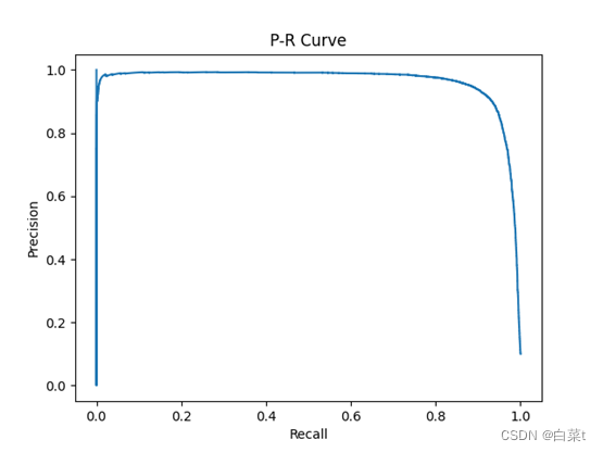
3.3.8 P-R图绘制

P-R图是获取预测结果中的每一个类别出现的所有概率，依次使用它们作为阈值来计算TP，TN，FP，FN。

TP：真实为真，预测的概率大于等于阈值；

FN：真实为真，预测小于阈值；

FP：真实为假，预测大于等于阈值；

TN：真实为假，预测小于阈值；

然后计算P和R。

可以使用sklearn.metrics的precision_recall_curve函数来计算P，R。average_precision_score计算平均精度(AP)。

平均精度(AP)，即在每个阈值处获得的精度的加权平均值，而前一个阈值的召回率增加用作权重：

$\text{AP} = \sum_{n}^{}{\left( R_{n} - R_{n - 1} \right)P_{n}}$

其中 $R_{n}$ 和 $P_{n}$ 是第n个阈值的精度和召回率。一对 ${(R_{k},\ \ P}_{k})$ 被成为称为操作点（operating point）。

step函数用于绘制阶梯图。

def step(self, x, y, *args, where=‘pre’, data=None, **kwargs):

cbook._check_in_list((‘pre’, ‘post’, ‘mid’), where=where)

kwargs[‘drawstyle’] = ‘steps-’ + where

return self.plot(x, y, *args, data=data, **kwargs)

step函数签名：

matplotlib.pyplot.step(x, y, *args, where=‘pre’, data=None, **kwargs)

step函数调用签名：

step(x, y, [fmt], *, data=None, where=‘pre’, **kwargs)

step(x, y, [fmt], x2, y2, [fmt2], …, *, where=‘pre’, **kwargs)

其中：

x：类数组结构，一维x轴坐标序列。一般假设x轴坐标均匀递增。必备参数。

y：类数组结构，一维y轴坐标序列。必备参数。

fmt：格式字符串，与plot函数的fmt参数类似。可选参数。官方建议只设置颜色格式。

data：可索引数据，类似于plot函数。可选参数。

**kwargs：类似于plot函数。

where ：设置阶梯所在位置，取值范围为{‘pre’, ‘post’,
‘mid’}，默认值为’pre’。

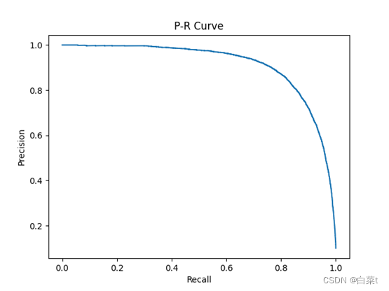
绘制总的P-R图：

Micro Average

微平均是指计算多分类指标时赋予所有类别的每个样本相同的权重，将所有样本合在一起计算各个指标。

precision = dict()
recall = dict()
average_precision = dict()
for i in range(10):
precision[i], recall[i], threshold = precision_recall_curve(y[:,
i],
res[:, i])
average_precision[i] = average_precision_score(y[:, i], res[:,
i])
# “micro-average”: quantifying score on all classes jointly
precision[“micro”], recall[“micro”], threshold =
precision_recall_curve(y.ravel(),
res.ravel())
average_precision[“micro”] = average_precision_score(y, res,
average=“micro”)

plt.step(recall[‘micro’], precision[‘micro’], where=‘post’)
plt.xlabel(‘Recall’)
plt.ylabel(‘Precision’)
plt.title(‘P-R Curve’)
plt.show()

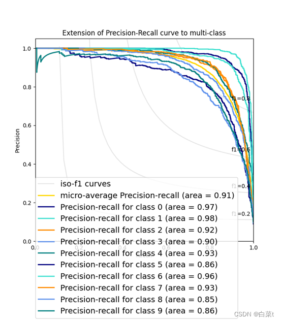
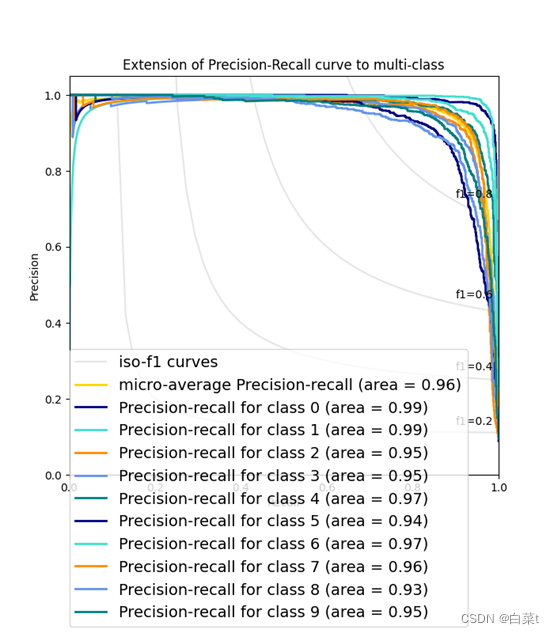
为每一个类和iso-f1曲线绘制P-R图：

from itertools import cycle
# 设置绘图细节
colors = cycle([‘navy’, ‘turquoise’, ‘darkorange’, ‘cornflowerblue’,
‘teal’])

plt.figure(figsize=(7, 8))
f_scores = np.linspace(0.2, 0.8, num=4)
lines = []
labels = []
l = []
for f_score in f_scores:
x = np.linspace(0.01, 1)
y = f_score * x / (2 * x - f_score)
l, = plt.plot(x[y >= 0], y[y >= 0], color=‘gray’, alpha=0.2)
plt.annotate(‘f1={0:0.1f}’.format(f_score), xy=(0.9, y[45] + 0.02))

lines.append(l)
labels.append(‘iso-f1 curves’)
l, = plt.plot(recall[“micro”], precision[“micro”], color=‘gold’,
lw=2)
lines.append(l)
labels.append(‘micro-average Precision-recall (area = {0:0.2f})’
‘’.format(average_precision[“micro”]))

for i, color in zip(range(10), colors):
l, = plt.plot(recall[i], precision[i], color=color, lw=2)
lines.append(l)
labels.append(‘Precision-recall for class {0} (area = {1:0.2f})’
‘’.format(i, average_precision[i]))

fig = plt.gcf()
fig.subplots_adjust(bottom=0.25)
plt.xlim([0.0, 1.0])
plt.ylim([0.0, 1.05])
plt.xlabel(‘Recall’)
plt.ylabel(‘Precision’)
plt.title(‘Extension of Precision-Recall curve to multi-class’)
plt.legend(lines, labels, loc=(0, -.38), prop=dict(size=14))

plt.show()

4 运行结果

4.1 一元线性回归训练结果图

真实直线为2*x+范围（-5,5）的随机数，iterations = 100000，lr =
0.000001。

在这里插入图片描述

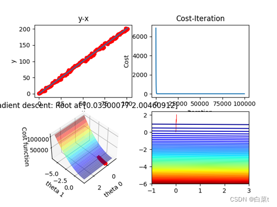
图1：可视化图，回归结果图，代价函数与迭代次数关系图，参数（w，b）与代价函数的三维关系图及二维登高线图

4.2 多元线性回归

进行了Standardization，把数据变为均值为0，方差为1的正态分布。

4.2.1梯度下降

使用ex2data1.txt数据集，iterations = 10000，lr = 0.01。

在这里插入图片描述

图2：cost-iteration图

回归模型评估：

theta:

[[ 2.25328063e+01]

[-9.28790471e-01]

[ 1.08215630e+00]

[ 1.39541876e-01]

[ 6.82628635e-01]

[-2.05849327e+00]

[ 2.67714841e+00]

[ 1.92553758e-02]

[-3.10722513e+00]

[ 2.66107374e+00]

[-2.07454109e+00]

[-2.06250627e+00]

[ 8.50082247e-01]

[-3.74718613e+00]]

$R^{2}:$ 0.7406426373989039

4.2.2公式法

使用Boston数据集，iterations = 10000，lr = 0.01。

theta:

[[ 2.25328063e+01]

[-9.29064566e-01]

[ 1.08263896e+00]

[ 1.41039433e-01]

[ 6.82414381e-01]

[-2.05875361e+00]

[ 2.67687661e+00]

[ 1.94853355e-02]

[-3.10711605e+00]

[ 2.66485220e+00]

[-2.07883689e+00]

[-2.06264585e+00]

[ 8.50108862e-01]

[-3.74733185e+00]]

$R^{2}:$0.7406426641094094

进程已结束,退出代码0

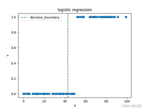
4.3 一元逻辑回归

4.3.1批量梯度下降

随机生成1-100之间的100个数，大于50的标签为1。iterations = 20000，lr =0.001。

在这里插入图片描述

图3：一元逻辑回归cost-iteration图

在这里插入图片描述

图4：一元逻辑回归数据图与决策边界图

4.3.2随机梯度下降

4.4 多元逻辑回归

使用mnist数据集，进行Standardization，把数据变为均值为0，方差为1的正态分布。

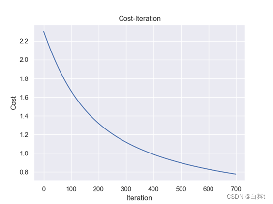
4.4.1批量梯度下降

iterations=700，lr=0.01，lamda=10。

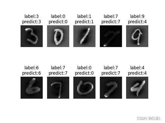
4.4.1.1 L1正则化

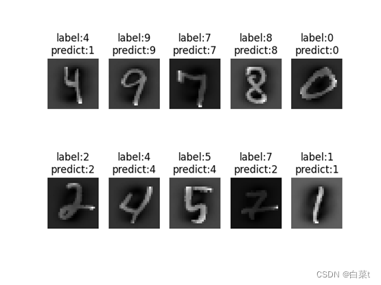
训练完后，随机抽取10张测试图片数据来预测展示。下图5-9分别为代价函数与迭代次数关系图，10张图片预测结果图，test数据集混淆矩阵，总体P-R曲线，各类P-R曲线。

在这里插入图片描述

图5：mnist数据集cost-interation图

在这里插入图片描述

图6：mnist数据集预测结果

在这里插入图片描述

图7：mnist数据集预测混淆矩阵

在这里插入图片描述

图8：mnist数据集总体P-R曲线

在这里插入图片描述

图9：mnist数据集各类P-R曲线

4.4.1.2 L2正则化

训练完后，随机抽取10张测试图片数据来预测展示。下图10-14分别为代价函数与迭代次数关系图，10张图片预测结果图，test数据集混淆矩阵，总体P-R曲线，各类P-R曲线。

在这里插入图片描述

图10：mnist数据集cost-interation图

在这里插入图片描述

图11：mnist数据集预测结果

在这里插入图片描述

图12：mnist数据集预测混淆矩阵

在这里插入图片描述

图13：mnist数据集总体P-R曲线

在这里插入图片描述

图14：mnist数据集各类P-R曲线

4.4.2随机梯度下降

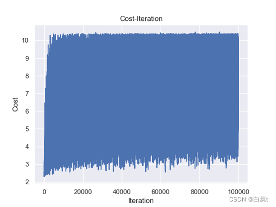
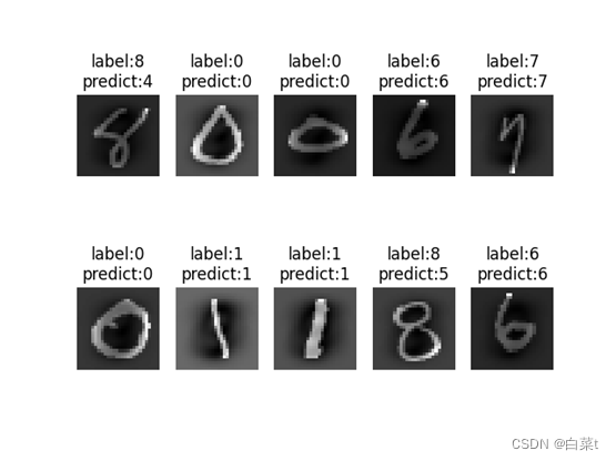
iterations = 100000，lr = 0.001，lamda = 10。

4.4.2.1 L1正则化

训练完后，随机抽取10张测试图片数据来预测展示。下图15-19分别为代价函数与迭代次数关系图，10张图片预测结果图，test数据集混淆矩阵，总体P-R曲线，各类P-R曲线。

在这里插入图片描述

图15：mnist数据集cost-interation图

在这里插入图片描述

图16：mnist数据集预测结果

在这里插入图片描述

图17：mnist数据集预测混淆矩阵

在这里插入图片描述

图18：mnist数据集总体P-R曲线

在这里插入图片描述

图19：mnist数据集各类P-R曲线

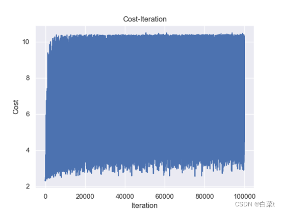
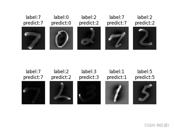
4.4.2.2 L2正则化

训练完后，随机抽取10张测试图片数据来预测展示。下图20-24分别为代价函数与迭代次数关系图，10张图片预测结果图，test数据集混淆矩阵，总体P-R曲线，各类P-R曲线。

在这里插入图片描述

图20：mnist数据集cost-interation图

在这里插入图片描述

图21：mnist数据集预测结果

在这里插入图片描述

图22：mnist数据集预测混淆矩阵

在这里插入图片描述

图23：mnist数据集总体P-R曲线

在这里插入图片描述

图24：mnist数据集各类P-R曲线

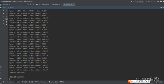
4.5 pytorch逻辑回归训练结果图

使用VehicleAttrs_V6数据集，batch_size = 4，num_epochs =
100，learning_rate = 0.01。总共训练100步，每个4张图片。

在这里插入图片描述

图25：训练结果

{width="5.768055555555556in"
height="3.066666666666667in"}

图26：预测结果

5 结论

特征缩放是将数据特征缩放到一定范围内，以使每个变量均对分析产生同等作用，数据进行特征缩放可以提升模型的精度和有效提高模型训练效率。

正则化的主要作用是防止过拟合，对模型添加正则化项可以限制模型的复杂度，使得模型在复杂度和性能达到平衡。回归模型评估可以有P，R，A，F1，P-R图，AP，mAP等。

遇到的问题和解决方法：
引入指数形式的缺点：指数函数的曲线斜率逐渐增大虽然能够将输出值拉开距离，但是也带来了缺点，当值非常大的话，计算得到的数值也会变的非常大，数值可能会溢出。当然针对数值溢出有其对应的优化方法，将每一个输出值减去输出值中最大的值。

Mnist数据集进行特征缩放时，std=np.std(train_x, axis=0,
ddof=1)是对列求标准差，可能为0，train_x /=
std会导致异常，需要将等于0的std赋值为1，不做变化。

线性回归和逻辑回归，或者BP神经网络计算，传入的单个参数必须是(1, )的。

模型的x，y参数不能是(n, )的形状，需要reshape(-1, 1)操作。

进行三维平面绘制时，传入的参数W，B原来是(n,1)的数组，必须转化为(n,)的数组，否则画三维平面和等高线会报错。

在SGD中，取了一个样本后， $x_{j}$ 形状是(1,)，必须改变形状为(1,
m)，不然会出错。

在SGD中，不能np.random.shuffle(train_x)
np.random.shuffle(train_y)这样独立地打乱x，y数据，要关联x，y。

indices = np.arange(len(train\_x))

np.random.shuffle(indices)

x\_shuffled = train\_x\[indices\]

y\_shuffled = train\_y\[indices\]

测试数据集应保持与训练数据集相同的特征缩放。模型是在训练数据集的缩放基础上进行训练的，如果测试数据集的缩放不一致，可能会影响模型的性能和预测结果的准确性。

6 程序源代码

6.1 一元线性回归

import numpy as np
import matplotlib.pyplot as plt


x = np.array(range(102))
# 加入随机噪声
noise = np.random.uniform(-5, 5, size=102)
# print(noise)
y = 2 * x
y = (y + noise).reshape(-1, 1)
x = np.reshape(x, (x.shape[0], 1))
x = np.insert(x, 0, 1, axis=1)
iterations = 100000
lr = 0.000001

theta = np.zeros([x.shape[-1], 1])
(n, m) = x.shape
costs = []
W = []
B = []


def model(x, theta):
    return np.dot(x, theta)


def cost(y_pre, y):
    return np.sum((y - y_pre) ** 2) / (2 * n)


def gradient_dscent(theta, iterations, lr):
    for i in range(iterations):
        y_pre = model(x, theta)

        dt = np.dot(x.T, (y_pre - y)) / n
        cst = cost(y_pre, y)

        costs.append(cst)
        theta = theta - lr * dt
        W.append(theta[1])
        B.append(theta[0])
        print("iteration:{}, cost={}".format(i, cst))
    return theta


theta = gradient_dscent(theta, iterations, lr)
y_pre = model(x, theta)
print(x[:, 1].shape, y_pre.shape)
fig = plt.figure()
plt.subplot(2, 2, 1)
plt.plot(x[:, 1], y_pre)
plt.scatter(x[:, 1], y, marker='o', c='r')
plt.ylabel('y')
plt.xlabel('x')
plt.title('y-x')
plt.subplot(2, 2, 2)
plt.plot(range(len(costs)), costs)
plt.xlabel('Iteration')
plt.ylabel('Cost')
plt.title('Cost-Iteration')

# 三维图和等高线
W = np.squeeze(W)  # 原来是(n,1)的数组，必须转化为(n,)的数组，否则会报错
B = np.squeeze(B)

# Setup of meshgrid of theta values
T0, T1 = np.meshgrid(np.linspace(-1, 3, 100), np.linspace(-6, 2, 100))

# Computing the cost function for each theta combination
zs = np.array([cost(model(x, np.array([t0, t1]).reshape(-1, 1)), y.reshape(-1, 1))
               for t0, t1 in zip(np.ravel(T0), np.ravel(T1))])
# Reshaping the cost values
Z = zs.reshape(T0.shape)
anglesx = np.array(B)[1:] - np.array(B)[:-1]
anglesy = np.array(W)[1:] - np.array(W)[:-1]
ax = fig.add_subplot(2, 2, 3, projection='3d')
ax.plot_surface(T0, T1, Z, rstride=5, cstride=5, cmap='jet', alpha=0.5)
ax.plot(B, W, costs, marker='*', color='r', alpha=.4, label='Gradient descent')

ax.set_xlabel('theta 0')
ax.set_ylabel('theta 1')
ax.set_zlabel('Cost function')
ax.set_title('Gradient descent: Root at {}'.format(theta.ravel()))
ax.view_init(45, 45)

# Contour plot
ax = fig.add_subplot(2, 2, 4)
ax.contour(T0, T1, Z, 70, cmap='jet')
ax.quiver(B[:-1], W[:-1], anglesx, anglesy, scale_units='xy', angles='xy', scale=1, color='r', alpha=.9)

plt.show()

6.2 多元线性回归

import numpy as np
import pandas as pd
import matplotlib.pyplot as plt
from sklearn.metrics import r2_score
df = pd.read_csv('Boston.csv', header=None)
data = np.array(df[1:]).astype(np.float64)
x = data[:, :-1]
y = data[:, -1]

y = np.reshape(y, (y.shape[0], 1))  # y原来是(100,)，要改变形状为(100, 1)，不然会出错
# print(x.shape, y.shape)
# 特征缩放 Standardization
x -= np.mean(x, axis=0)
x /= np.std(x, axis=0, ddof=1)
x = np.insert(x, 0, 1, axis=1)
iterations = 10000
lr = 0.01

theta = np.zeros([x.shape[-1], 1])
(n, m) = x.shape
costs = []


def model(x, theta):
    return np.dot(x, theta)


def cost(y_pre, y):
    return np.sum((y - y_pre) ** 2) / (2 * n)


def gradient_dscent(theta, iterations, lr):
    for i in range(iterations):
        y_pre = model(x, theta)

        dt = np.dot(x.T, (y_pre - y)) / n
        cst = cost(y_pre, y)

        costs.append(cst)
        theta = theta - lr * dt
        print("iteration:{}, cost={}".format(i, cst))
    return theta


def get_theta(theta, x, y):
    return np.dot(np.linalg.inv(np.dot(x.T, x)), np.dot(x.T, y))


theta = gradient_dscent(theta, iterations, lr)
# theta = get_theta(theta, x, y)
print(theta)
y_pre = model(x, theta)
ss_tot = np.sum((y-np.mean(y))**2)
ss_reg = np.sum((y_pre-np.mean(y))**2)
ss_res = np.sum((y-y_pre)**2)
r_sq = 1-ss_res/ss_tot
print(r_sq)
# score = r2_score(y, y_pre) 回归系数，上面为具体求解过程
plt.plot(range(len(costs)), costs)
plt.xlabel('Iteration')
plt.ylabel('Cost')
plt.title('Cost-Iteration')
plt.show()

6.3 一元逻辑回归

import numpy as np
import matplotlib.pyplot as plt

# 生成随机数据作为自变量 x
x = np.random.uniform(0, 100, 100)
y = (x > 50).astype(np.int32)  # 将布尔值转换为 0 和 1
# print(y.shape)
x = x.reshape(100, -1)
y = y.reshape(100, -1)  # y原来是(100,)，要改变形状为(100, 1)，不然会出错
# 特征缩放 Standardization
# x -= np.mean(x, axis=0)
# x /= np.std(x, axis=0, ddof=1)
x = np.insert(x, 0, 1, axis=1)
# print(x)
# print(y)
iterations = 100000
lr = 0.0001
theta = np.zeros([x.shape[-1], 1])
(n, m) = x.shape
costs = []


def sigmod(z):
    return 1.0 / (1 + np.exp(-z))


def model(x, theta):
    return np.dot(x, theta)


def cost(y_pre, y):
    return -np.sum(y * np.log(y_pre + 1e-5) + (1 - y) * np.log(1 - y_pre + 1e-5)) / n


def gradient_dscent(theta, iterations, lr, gd_type):
    if gd_type == 1:
        for i in range(iterations):
            z = model(x, theta)
            y_pre = sigmod(z)
            dt = np.dot(x.T, (y_pre - y)) / n
            cst = cost(y_pre, y)
            costs.append(cst)
            theta = theta - lr * dt
            print("iteration:{}, cost={}".format(i, cst))
    elif gd_type == 2:  # 随机
        j = 0
        indices = np.arange(len(x))
        np.random.shuffle(indices)
        x_shuffled = x[indices]
        y_shuffled = y[indices]
        for i in range(iterations):
            x_j = np.reshape(x_shuffled[j], (1, x_shuffled.shape[1]))  # x_j原来是(1,)，要改变形状为(1, m)，不然会出错
            y_j = y_shuffled[j]
            z_j = model(x_j, theta)
            y_pre_j = sigmod(z_j)
            dt_j = np.dot(x_j.T, (y_pre_j - y_j))
            cst = cost(y_pre_j, y_shuffled)
            costs.append(cst)
            theta = theta - lr * dt_j
            j += 1
            if j >= n:
                j = 0
                indices = np.arange(len(x))
                np.random.shuffle(indices)
                x_shuffled = x[indices]
                y_shuffled = y[indices]
            if i % 100 == 0:
                print("iteration:{}, cost={}".format(i, cst))
    return theta


def evaluate_model(x, y, theta):
    y_pre = sigmod(model(x, theta))
    res = np.hstack((1-y_pre, y_pre))
    y_pre = np.argmax(res, axis=1)
    print(theta)
    TP = 0
    FP = 0
    FN = 0
    TN = 0
    for i in range(len(y)):
        if y_pre[i] == 0 and y[i] == 0:
            TP += 1
        elif y_pre[i] == 0 and y[i] == 1:
            FP += 1
        elif y_pre[i] == 1 and y[i] == 0:
            FN += 1
        elif y_pre[i] == 1 and y[i] == 1:
            TN += 1
    print(TP, FP, FN, TN)
    percision = TP / (TP + FP)
    accuracy = (TP + TN) / (TP + FP + FN + TN)
    recall = TP / (TP + FN)
    F1 = 2*percision*recall/(percision+recall)
    confu_mat = np.array([[TP, FN], [FP, TN]]).reshape(2, 2)
    print("confuse matrix:\n", confu_mat)
    print("percision={}, accuracy={}, recall={}, F1={}".format(percision, accuracy, recall, F1))


theta = gradient_dscent(theta, iterations, lr, 2)
w = theta[1]
b = theta[0]
evaluate_model(x, y, theta)
plt.plot(range(len(costs)), costs)
plt.xlabel('Iteration')
plt.ylabel('Cost')
plt.title('Cost-Iteration')
plt.show()
decision_boundary = -b / w
print(decision_boundary)


# 绘制散点图和决策边界
plt.scatter(x[:, 1], y)
plt.axvline(x=decision_boundary, color='green', linestyle='--', label='decision_boundary')
plt.legend()
plt.xlabel('X')
plt.ylabel('Y')
plt.title('logistic regression')
plt.show()

6.4 多元逻辑回归

import numpy as np
import tensorflow as tf
from matplotlib import pyplot as plt
from sklearn.metrics import confusion_matrix, precision_recall_curve, average_precision_score
import seaborn as sns

k = 10
mnist = tf.keras.datasets.mnist
(train_x, train_y), (test_x, test_y) = mnist.load_data()
train_y = np.eye(k)[train_y]
test_y = np.eye(k)[test_y]

train_x = train_x.astype(np.float64) / 255.0
test_x = test_x.astype(np.float64) / 255.0
train_x = train_x.reshape(train_x.shape[0], -1)
test_x = test_x.reshape(test_x.shape[0], -1)

# print(np.mean(train_x, axis=0))
# # 特征缩放 Standardization
train_x -= np.mean(train_x, axis=0)
std_dev = np.std(train_x, axis=0, ddof=1)
std_dev[std_dev == 0] = 1  # 将为0的标准差替换为1
train_x /= std_dev
train_x = np.insert(train_x, 0, 1, axis=1)

# 测试数据集应保持与训练数据集相同的缩放。模型是在训练数据集的缩放基础上进行训练的，如果测试数据集的缩放不一致，可能会影响模型的性能和预测结果的准确性。
test_x -= np.mean(test_x, axis=0)
std_dev = np.std(test_x, axis=0, ddof=1)
std_dev[std_dev == 0] = 1  # 将为0的标准差替换为1
test_x /= std_dev
test_x = np.insert(test_x, 0, 1, axis=1)

print('train_x:%s, train_y:%s, test_x:%s, test_y:%s' % (train_x.shape, train_y.shape, test_x.shape, test_y.shape))

iterations = 100000
lr = 0.001
lamda = 10
theta = np.zeros([train_x.shape[-1], 10])
(n, m) = train_x.shape
costs = []


def softmax(Z):
    row_max = np.max(Z, axis=1)  # 每行的最大值 axis=1是每一行的所有元素之和
    row_max = row_max.reshape(-1, 1)
    Z = Z - row_max
    Z_exp = np.exp(Z)
    Z_exp_sum = np.sum(Z_exp, axis=1, keepdims=True)
    return Z_exp / Z_exp_sum


def model(x, theta):
    return np.dot(x, theta)


def cost(y_pre, y):
    return -np.sum(y * np.log(y_pre + 1e-5)) / n


def gradient_dscent(theta, iterations, lr, lamda, gd_type=1, reg_type=1):
    if gd_type == 1:  # 批量
        for i in range(iterations):
            # print(train_x.shape, theta.shape)
            z = model(train_x, theta)
            # print(z[0])
            y_pre = softmax(z)
            dt = np.dot(train_x.T, (y_pre - train_y)) / n
            cst = cost(y_pre, train_y)
            if reg_type == 2:  # l2
                cst += lamda / (2 * n) * np.sum(theta ** 2)
                costs.append(cst)
                dt += lamda / n * theta
            elif reg_type == 1:  # l1
                cst += lamda / (2 * n) * np.sum(np.abs(theta))
                costs.append(cst)
                dt += lamda / n * np.sign(theta)
            theta = theta - lr * dt
            if i % 100 == 0:
                print("Cost after iteration %i: %f" % (i, cst))
    elif gd_type == 2:  # 随机
        j = 0
        indices = np.arange(len(train_x))
        np.random.shuffle(indices)
        x_shuffled = train_x[indices]
        y_shuffled = train_y[indices]
        for i in range(iterations):
            x_j = np.reshape(x_shuffled[j], (1, x_shuffled.shape[1]))  # x_j原来是(1,)，要改变形状为(1, m)，不然会出错
            y_j = y_shuffled[j]
            z_j = model(x_j, theta)
            y_pre_j = softmax(z_j)
            dt_j = np.dot(x_j.T, (y_pre_j - y_j))
            cst = cost(y_pre_j, y_shuffled)
            if reg_type == 2:  # l2
                cst += lamda / (2 * n) * np.sum(theta ** 2)
                costs.append(cst)
                dt_j += lamda / n * theta
            elif reg_type == 1:  # l1
                cst += lamda / (2 * n) * np.sum(np.abs(theta))
                costs.append(cst)
                dt_j += lamda / n * np.sign(theta)
            theta = theta - lr * dt_j
            j += 1
            if j >= n:
                j = 0
                indices = np.arange(len(train_x))
                np.random.shuffle(indices)
                x_shuffled = train_x[indices]
                y_shuffled = train_y[indices]
            if i % 100 == 0:
                print("Cost after iteration %i: %f" % (i, cst))
    return theta


def evaluate_model(x, y, theta):
    print(y.shape)
    Y_out = np.zeros([x.shape[0], y.shape[1]])

    res = softmax(model(x, theta))
    # print(res)
    idx = np.argmax(res, axis=1)
    Y_out[range(y.shape[0]), idx] = 1
    acc = np.sum(Y_out * y) / y.shape[0]
    print("Training accuracy is: %f" % acc)

    for i in range(10):
        num = np.random.randint(1, 10000)
        plt.subplot(2, 5, i + 1)
        plt.axis('off')
        plt.imshow(test_x[num, 1:].reshape(28, 28), cmap='gray')
        y_pre = softmax(model(test_x[num], theta).reshape(1, 10))
        y_pred = np.argmax(y_pre)
        # print(model(test_x[num], theta).reshape(1, 10))
        print(y_pre)
        plt.title('label:' + str(np.argmax(test_y[num])) + '\npredict:' + str(y_pred))
    plt.show()

    # label_y = np.argmax(y, axis=1)  # 混淆矩阵的求法，但是这个太慢了
    # for k in range(y.shape[0]):
    #     for i in range(m):
    #         for j in range(m):
    #             cm[i, j] += ((idx[k] == i) == (label_y[k] == j))

    # label_y = np.argmax(y, axis=1)
    # 求混淆矩阵的快速方法
    # # 使用bincount方法计算每个类别组合的频次
    # # 需要将 idx 和 label_y 转换为一维数组
    # # 然后使用 m * label_y + idx 来获取每个元素的唯一索引
    # cm_flat = np.bincount(k * label_y + idx, minlength=k * k)
    # # 将一维数组重新变形为 k x k 的矩阵
    # cm = cm_flat.reshape(k, k)

    label_y = np.argmax(y, axis=1)
    cm = confusion_matrix(label_y, idx, labels=[0, 1, 2, 3, 4, 5, 6, 7, 8, 9])  # 使用库
    print("confusion matrix:\n", cm)
    # print(cm.shape)
    TP = np.diag(cm)  # 真阳性
    FP = cm.sum(axis=0) - TP  # 假阳性
    FN = cm.sum(axis=1) - TP  # 假阴性
    # TN = cm.sum() - (FP + FN + TP)  # 真阴性,用不到

    precision = dict()
    recall = dict()
    average_precision = dict()
    for i in range(10):
        precision[i], recall[i], threshold = precision_recall_curve(y[:, i],
                                                                    res[:, i])
        average_precision[i] = average_precision_score(y[:, i], res[:, i])
    # "micro-average": quantifying score on all classes jointly
    precision["micro"], recall["micro"], threshold = precision_recall_curve(y.ravel(),
                                                                            res.ravel())
    average_precision["micro"] = average_precision_score(y, res,
                                                         average="micro")
    from itertools import cycle
    # 设置绘图细节
    colors = cycle(['navy', 'turquoise', 'darkorange', 'cornflowerblue', 'teal'])

    plt.figure(figsize=(7, 8))
    f_scores = np.linspace(0.2, 0.8, num=4)
    lines = []
    labels = []
    l = []
    for f_score in f_scores:
        x = np.linspace(0.01, 1)
        y = f_score * x / (2 * x - f_score)
        l, = plt.plot(x[y >= 0], y[y >= 0], color='gray', alpha=0.2)
        plt.annotate('f1={0:0.1f}'.format(f_score), xy=(0.9, y[45] + 0.02))

    lines.append(l)
    labels.append('iso-f1 curves')
    l, = plt.plot(recall["micro"], precision["micro"], color='gold', lw=2)
    lines.append(l)
    labels.append('micro-average Precision-recall (area = {0:0.2f})'
                  ''.format(average_precision["micro"]))

    for i, color in zip(range(10), colors):
        l, = plt.plot(recall[i], precision[i], color=color, lw=2)
        lines.append(l)
        labels.append('Precision-recall for class {0} (area = {1:0.2f})'
                      ''.format(i, average_precision[i]))

    fig = plt.gcf()
    fig.subplots_adjust(bottom=0.25)
    plt.xlim([0.0, 1.0])
    plt.ylim([0.0, 1.05])
    plt.xlabel('Recall')
    plt.ylabel('Precision')
    plt.title('Extension of Precision-Recall curve to multi-class')
    plt.legend(lines, labels, loc=(0, -.38), prop=dict(size=14))

    plt.show()

    plt.step(recall['micro'], precision['micro'], where='post')
    plt.xlabel('Recall')
    plt.ylabel('Precision')
    plt.title('P-R Curve')
    plt.show()

    precision = np.mean(TP / (TP + FP))
    accuracy = TP.sum() / cm.sum()
    recall = np.mean(TP / (TP + FN))
    F1 = np.mean(2 * (precision * recall) / (precision + recall))

    print("precision={}, accuracy={}, recall={}, F1={}".format(precision, accuracy, recall, F1))

    sns.set()
    sns.heatmap(cm, cmap='Reds', linewidths=0.1, linecolor='white', square=True, annot=True, fmt='g')
    plt.xlabel('predict')
    plt.ylabel('label')
    plt.title('confusion_matrix')
    plt.show()


theta = gradient_dscent(theta, iterations, lr, lamda, 2, 2)
evaluate_model(test_x, test_y, theta)
plt.plot(range(len(costs)), costs)
plt.xlabel('Iteration')
plt.ylabel('Cost')
plt.title('Cost-Iteration')
plt.show()

6.5 使用pytorch库进行逻辑回归

train.py

import torch
import numpy as np
import torchvision
from matplotlib import pyplot as plt
from torch import nn
from torch.utils.data import DataLoader
from torchvision import transforms
from torchvision import datasets
import torch.nn.functional as F

from model import LR

# 特征缩放 数据集转换为tensor格式
transform = transforms.Compose(
    [transforms.Resize((320, 320)), transforms.ToTensor(), transforms.Normalize((0.1307,), (0.3081,))])

# 数据集路径
train_data_dir = r'E:\BaiduNetdiskDownload\VehicleAttrs_V6\train'
test_data_dir = r'E:\BaiduNetdiskDownload\VehicleAttrs_V6\val'

batch_size = 4
num_epochs = 100
num_classes = 10
learning_rate = 0.01

# 获取数据集
train_dataset = datasets.ImageFolder(root=train_data_dir, transform=transform)
test_dataset = datasets.ImageFolder(root=test_data_dir, transform=transform)

# 输出类别标签与数字的映射结果
for class_idx, class_label in enumerate(train_dataset.classes):
    print(f'Class Label: {class_label}, Numeric Label: {class_idx}')
# Result:
#     Class Label: bus, Numeric Label: 0
#     Class Label: fuel, Numeric Label: 1
#     Class Label: mpv, Numeric Label: 2
#     Class Label: pickup, Numeric Label: 3
#     Class Label: sedan, Numeric Label: 4
#     Class Label: suv, Numeric Label: 5
#     Class Label: truck, Numeric Label: 6


# Class Label: SUV, Numeric Label: 0
# Class Label: bus, Numeric Label: 1
# Class Label: family sedan, Numeric Label: 2
# Class Label: fire engine, Numeric Label: 3
# Class Label: heavy truck, Numeric Label: 4
# Class Label: jeep, Numeric Label: 5
# Class Label: minibus, Numeric Label: 6
# Class Label: racing car, Numeric Label: 7
# Class Label: taxi, Numeric Label: 8
# Class Label: truck, Numeric Label: 9
# 数据集加载
# 数据加载器（dataloader ）实例化一个dataset后，然后用Dataloader包起来，即载入数据集。shuffle=True即打乱数据集，打乱训练集进行训练，而对测试集进行顺序测试。
train_loader = torch.utils.data.DataLoader(dataset=train_dataset, batch_size=batch_size, shuffle=True)
test_loader = torch.utils.data.DataLoader(dataset=test_dataset, batch_size=batch_size, shuffle=False)

# 参数设置
input_size = 102400 * 3
total_step = len(train_loader)

# 定义模型
LR_model = LR(input_size, num_classes)

# 定义逻辑回归的损失函数，采用nn.CrossEntropyLoss(),nn.CrossEntropyLoss()内部集成了softmax函数
criterion = nn.CrossEntropyLoss(reduction='mean')

# 定义优化器
# optimizer = torch.optim.SGD(LR_model.parameters(), lr=learning_rate)
optimizer = torch.optim.Adam(LR_model.parameters(), lr=learning_rate)

# 训练模型-------------------------------------------------------------------------------------------------------------------------
# 定义保存路径和文件名的格式
save_path_format = 'runs/model_epoch_{}.ckpt'
for epoch in range(num_epochs):
    LR_model.train()
    for i, (images, labels) in enumerate(train_loader):

        # 将图像序列转换至大小为 (batch_size, input_size)
        images = images.reshape(-1, 320 * 320 * 3)

        # forward
        y_pred = LR_model(images)
        # print(y_pred.size())
        # print(labels.size())
        loss = criterion(y_pred, labels)

        # backward()
        optimizer.zero_grad()
        loss.backward()
        optimizer.step()
        if (i % (total_step - 1) == 0):
            print('Epoch [{}/{}], Step [{}/{}], Loss: {:.4f}'.format(epoch + 1, num_epochs, i + 1, total_step,
                                                                     loss.item()))

            # 验证模型---------------------------------------------------------
            # PyTorch 默认每一次前向传播都会计算梯度
            with torch.no_grad():
                correct = 0
                total = 0
                val_loss = 0
                for images, labels in test_loader:
                    images = images.reshape(-1, 320 * 320 * 3)
                    outputs = LR_model(images)
                    loss = criterion(outputs, labels)
                    val_loss += loss.item()
                    # torch.max的输出：out (tuple, optional) – the result tuple of two output tensors (max, max_indices)
                    max, predicted = torch.max(outputs.data, 1)
                    # print(max.data)
                    # print(predicted)
                    total += labels.size(0)
                    correct += (predicted == labels).sum()

                print('Accuracy of the model on test dataset: {} %'.format(100 * correct / total))
                # print('Average val loss of the model on test dataset: {} '.format(val_loss / len(test_loader)))

            ## 保存模型
            save_path = save_path_format.format(epoch + 1)
            torch.save(LR_model.state_dict(), save_path)
            # torch.save(LR_model.state_dict(), 'model.ckpt')

print("Training finished.")

model.py

import torch
import torch.nn as nn
import torch.nn.functional as F


# 定义逻辑回归模型
class LR(nn.Module):
    def __init__(self, input_dims, output_dims):
        super().__init__()
        self.linear = nn.Linear(input_dims, output_dims, bias=True)

    def forward(self, x):
        x = self.linear(x)
        # x = F.sigmoid(x)
        return x

白菜t

关注

23
点赞
踩
22

收藏

觉得还不错? 一键收藏
0
评论
线性回归与逻辑回归

1 设计内容与要求 2 实验环境 2.1 硬件环境： 2.2 软件环境： 3 系统分析与设计 3.1 系统功能需求分析 3.1.1 数据集的选择 3.1.2 算法选择 3.1.2.1 梯度下降 3.1.2.2 公式法 3.1.3 特征缩放 3.1.4 正则化 3.1.5 可视化方法 3.1.6 模型评估 3.1.7 性能需求 3.2 系统结构图 3.3 关键技术难点的实现 3.3.1 线性回归模型构造 3.3.1.1线性回归 3.3.1.2逻辑回归 3.3.2 TP、FP、TN及FN的取值 3.3.4 混淆
复制链接

扫一扫