计算机视觉——SIFT特征提取算法

最新推荐文章于 2025-09-14 21:39:13 发布

原创最新推荐文章于 2025-09-14 21:39:13 发布 · 3.5k 阅读

CC 4.0 BY-SA版权

本文详细介绍了SIFT特征提取算法，包括算法简介、特点、应用场景。SIFT算法在旋转、缩放、光照变化等条件下保持稳定，适用于图像匹配和检索。实验表明，SIFT在精确性上优于Harris算法，但速度较慢。文中还探讨了匹配结果、图库检索以及RANSAC算法在图像拼接中的应用，并分享了遇到的问题及解决方案。

1. SIFT特征提取算法

1.1 算法简介

尺度不变特征转换(Scale-invariant feature transform或SIFT)是一种电脑视觉的算法用来侦测与描述影像中的局部性特征，它在空间尺度中寻找极值点，并提取出其位置、尺度、旋转不变量，此算法由 David Lowe在1999年所发表，2004年完善总结。
SIFT算法的实质是在不同的尺度空间上查找关键点(特征点)，并计算出关键点的方向。SIFT所查找到的关键点是一些十分突出，不会因光照，仿射变换和噪音等因素而变化的点，如角点、边缘点、暗区的亮点及亮区的暗点等。

1.2 特点介绍

SIFT特征是图像的局部特征，其对旋转、尺度缩放、亮度变化保持不变性，对视角变化、仿射变换、噪声也保持一定程度的稳定性；
独特性（Distinctiveness）好，信息量丰富，适用于在海量特征数据库中进行快速、准确的匹配；
多量性，即使少数的几个物体也可以产生大量的SIFT特征向量；
高速性，经优化的SIFT匹配算法甚至可以达到实时的要求；
可扩展性，可以很方便的与其他形式的特征向量进行联合。

1.3 算法可解决的问题

目标的自身状态、场景所处的环境和成像器材的成像特性等因素影响图像配准/目标识别跟踪的性能。而SIFT算法在一定程度上可解决：

目标的旋转、缩放、平移（RST）
图像仿射/投影变换（视点viewpoint）
光照影响（illumination）
目标遮挡（occlusion）
杂物场景（clutter）
噪声

2. 检测提取感兴趣点

2.1 检测结果

原图：
在这里插入图片描述
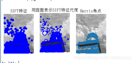
检测结果：

2.2 实验小结

从上面实验结果来看，harris算法在图像变换次数较多的情况下相比于sift算法提取特征点坐标偏移量相对较小。即sift算法更加精确，位置更加明确，但是算法运行速度比起harris算法来说更慢。

2.3 代码

# -*- coding: utf-8 -*-
from PIL import Image
from pylab import *
from PCV.localdescriptors import sift
from PCV.localdescriptors import harris

# 添加中文字体支持
from matplotlib.font_manager import FontProperties
font = FontProperties(fname=r"c:\windows\fonts\SimSun.ttc", size=14)

imname = 'E:/python/ttwst/picture/24.jpg'
im = array(Image.open(imname).convert('L'))
sift.process_image(imname, 'empire.sift')
l1, d1 = sift.read_features_from_file('empire.sift')

figure()
gray()
subplot(131)
sift.plot_features(im, l1, circle=False)
title(u'SIFT特征',fontproperties=font)
subplot(132)
sift.plot_features(im, l1, circle=True)
title(u'用圆圈表示SIFT特征尺度',fontproperties=font)

# 检测harris角点
harrisim = harris.compute_harris_response(im)

subplot(133)
filtered_coords = harris.get_harris_points(harrisim, 6, 0.1)
imshow(im)
plot([p[1] for p in filtered_coords], [p[0] for p in filtered_coords], '*')
axis('off')
title(u'Harris角点',fontproperties=font)

show()

3. 图片进行SIFT匹配

3.1 匹配结果

在这里插入图片描述

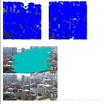
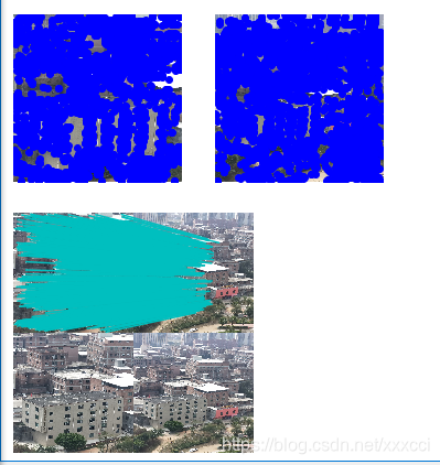
图片差异大时：

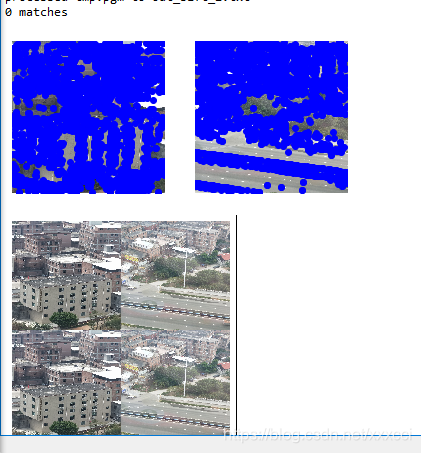
3.2 实验小结

对于将一幅图像中的特征匹配到另一幅图像的特征，一种稳健的准则是使用这两个特征距离和两个最匹配特征距离的比率，该准则保证能够找到足够相似的唯一特征。因为SIFT算法具有尺度和旋转不变性，所以图片即使角度不同也能找出共同特征点。

3.3 代码

from PIL import Image
from pylab import *
import sys
from PCV.localdescriptors import sift


if len(sys.argv) >= 3:
  im1f, im2f = sys.argv[1], sys.argv[2]
else:
#  im1f = '../data/sf_view1.jpg'
#  im2f = '../data/sf_view2.jpg'
  im1f = 'E:/python/ttwst/picture/1.jpg'
  im2f = 'E:/python/ttwst/picture/2.jpg'
#  im1f = '../data/climbing_1_small.jpg'
#  im2f = '../data/climbing_2_small.jpg'
im1 = array(Image.open(im1f))
im2 = array(Image.open(im2f))

sift.process_image(im1f, 'out_sift_1.txt')
l1, d1 = sift.read_features_from_file('out_sift_1.txt')
figure()
gray()
subplot(121)
sift.plot_features(im1, l1, circle=False)

sift.process_image(im2f, 'out_sift_2.txt')
l2, d2 = sift.read_features_from_file('out_sift_2.txt')
subplot(122)
sift.plot_features(im2, l2, circle=False)

#matches = sift.match(d1, d2)
matches = sift.match_twosided(d1, d2)
print ('{} matches'.format(len(matches.nonzero()[0])))

figure()
gray()
sift.plot_matches(im1, im2, l1, l2, matches, show_below=True)
show()

4. 图库检索图片匹配

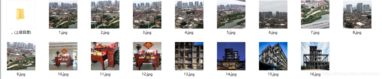
4.1 数据集

在这里插入图片描述

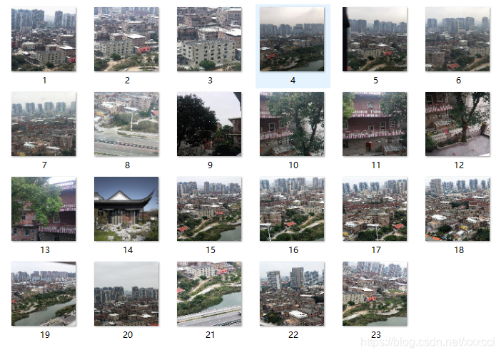
4.2 检索结果

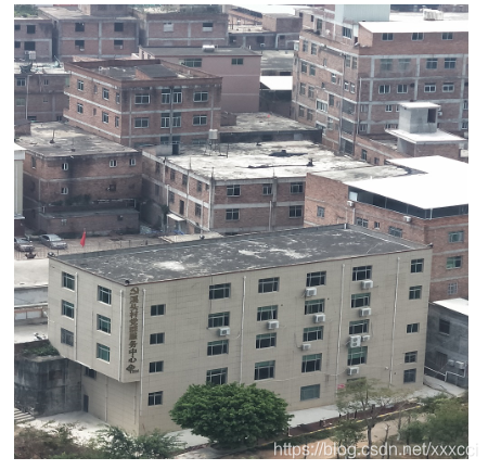
待检测图像：
在这里插入图片描述
检测结果：

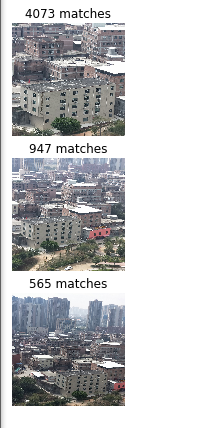
4.3 实验小结

在进行匹配时发现，如果图片太大会导致检测速度过慢以及电脑死机的情况，所以将图片调小了使得检测速度快一点，并且像素都一样。输入图片后，即在数据集中搜索到特征点相似最高的前三项，并且sift算法在大量数据中计算也非常快。
总的来说，匹配前三的精度还可以，但是运行速度有待提高，即使我已经把图片调的只有几百k，5m以上的图片就要死机。但是sift算法能排除对于颜色光照等影响，精确的匹配出相似度高的图片。

4.4 代码

from PIL import Image
from pylab import *
from PCV.localdescriptors import sift
import matplotlib.pyplot as plt


im1f = 'E:/python/ttwst/picture/new1/3.jpg'
im1 = array(Image.open(im1f))
sift.process_image(im1f, 'out_sift_1.txt')
l1, d1 = sift.read_features_from_file('out_sift_1.txt')

arr=[]
arrHash = {}
for i in range(1,23):

    im2f = (r'E:/python/ttwst/picture/new1/'+str(i)+'.jpg')
    im2 = array(Image.open(im2f))
    sift.process_image(im2f, 'out_sift_2.txt')
    l2, d2 = sift.read_features_from_file('out_sift_2.txt')
    matches = sift.match_twosided(d1, d2)
    length=len(matches.nonzero()[0])
    length=int(length)
    arr.append(length)
    arrHash[length]=im2f

arr.sort()
arr=arr[::-1]
arr=arr[:3]
i=0
plt.figure(figsize=(5,12))
for item in arr:
    if(arrHash.get(item)!=None):
        img=arrHash.get(item)
        im1 = array(Image.open(img))
        ax=plt.subplot(511 + i)
        ax.set_title('{} matches'.format(item))
        plt.axis('off')
        imshow(im1)
        i = i + 1

plt.show()

5. 实验遇到的问题及解决办法

5.1 找不到sift文件

一开始是在pycharm上面运行的，但是pycharm上面不论我修改了cmmd路径或是更改别的设置始终显示找不到sift.py文件，后来我改在spyder上面运行就没有这个问题。

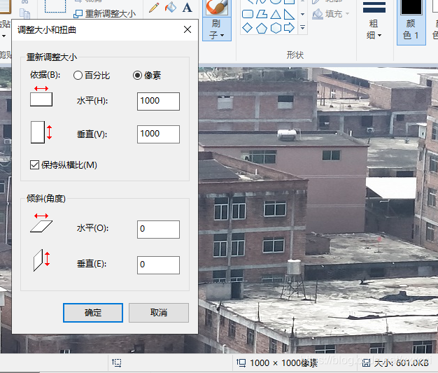
5.2 运行结果出不来

在运行两图片匹配时，一开始没有修改图片大小，两张图片一个5.0M一个4.8M太大了导致电脑直接死机，后来在编辑器中修改了图片的像素大小使得图片只有几百k就可以运行了。并且我将所有的图片都改成1000*1000，就不会出现像素不匹配的情况。
在这里插入图片描述

5.3 整数浮点数错误

在改完前面错误后发现出现IndexError:
在这里插入图片描述
百度显示是错误运用浮点数，我向同学要了sity.py文件，将自己的文件替换就不会报错了。

6. 地理标记图像匹配

6.1 代码

# -*- coding: utf-8 -*-
from pylab import *
from PIL import Image
from PCV.localdescriptors import sift
from PCV.tools import imtools
import pydot

""" This is the example graph illustration of matching images from Figure 2-10.
To download the images, see ch2_download_panoramio.py."""

#download_path = "panoimages"  # set this to the path where you downloaded the panoramio images
#path = "/FULLPATH/panoimages/"  # path to save thumbnails (pydot needs the full system path)

download_path = "E:/python/ttwst/picture/new1"  # set this to the path where you downloaded the panoramio images
path = "E:/python/ttwst/picture/new1/"  # path to save thumbnails (pydot needs the full system path)

# list of downloaded filenames
imlist = imtools.get_imlist(download_path)
nbr_images = len(imlist)

# extract features
featlist = [imname[:-3] + 'sift' for imname in imlist]
for i, imname in enumerate(imlist):
    sift.process_image(imname, featlist[i])

matchscores = zeros((nbr_images, nbr_images))

for i in range(nbr_images):
    for j in range(i, nbr_images):  # only compute upper triangle
        print ('comparing ', imlist[i], imlist[j])
        l1, d1 = sift.read_features_from_file(featlist[i])
        l2, d2 = sift.read_features_from_file(featlist[j])
        matches = sift.match_twosided(d1, d2)
        nbr_matches = sum(matches > 0)
        print ('number of matches = ', nbr_matches)
        matchscores[i, j] = nbr_matches
print ("The match scores is: \n", matchscores)

# copy values
for i in range(nbr_images):
    for j in range(i + 1, nbr_images):  # no need to copy diagonal
        matchscores[j, i] = matchscores[i, j]

#可视化

threshold = 2  # min number of matches needed to create link

g = pydot.Dot(graph_type='graph')  # don't want the default directed graph

for i in range(nbr_images):
    for j in range(i + 1, nbr_images):
        if matchscores[i, j] > threshold:
            # first image in pair
            im = Image.open(imlist[i])
            im.thumbnail((100, 100))
            filename = path + str(i) + '.jpg'
            im.save(filename)  # need temporary files of the right size
            g.add_node(pydot.Node(str(i), fontcolor='transparent', shape='rectangle', image=filename))

            # second image in pair
            im = Image.open(imlist[j])
            im.thumbnail((100, 100))
            filename = path + str(j) + '.jpg'
            im.save(filename)  # need temporary files of the right size
            g.add_node(pydot.Node(str(j), fontcolor='transparent', shape='rectangle', image=filename))

            g.add_edge(pydot.Edge(str(i), str(j)))
g.write_png('whitehouse.jpg')

6.2 运行结果

在这里插入图片描述

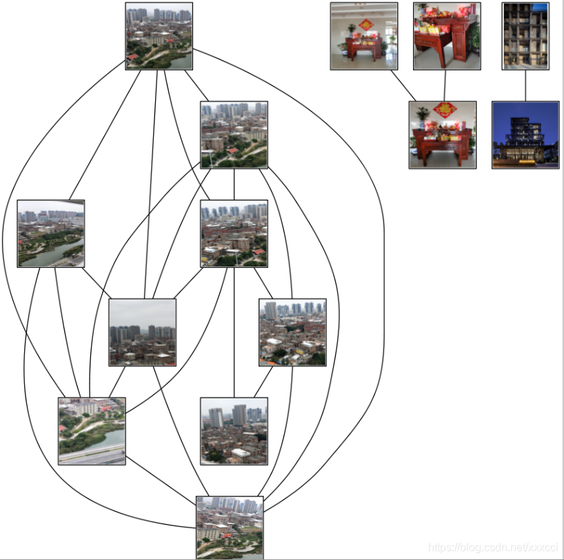
6.3 结果分析

上面结果是先经过局部描述子匹配，将两两图像间的匹配特征数保存在matchscores数组中，最后一部分将矩阵填充完整，但是可以不通过复制数值来填充完整，填充完整只是为了更好看，原因是该“距离度量”矩阵是对称的。这个矩阵就是图像间的距离度量方式。
矩阵对应位置的数据不为0即表示有匹配的特征点，若为0则表示不匹配。
这个算法是穷举法，我准备了16张图，两两之间都要匹配，所以次数非常多，一次匹配大概是30秒，总的运行时间将近一个半小时，非常久，但是不知道是什么原因，也许图片还是不够小。
我的图片包含建筑群，房屋，马路，还有湖，在测试过程中我发现建筑群这种特征明显的图像匹配值更多，而且有的图片人眼观察是觉得匹配的但是运行结果没有显示，有可能是因为特征不够明显。

7. RANSAC算法

7.1 算法介绍

RANSAC算法的输入是一组观测数据，一个可以解释或者适应于观测数据的参数化模型，一些可信的参数。
RANSAC通过反复选择数据中的一组随机子集来达成目标。被选取的子集被假设为局内点，并用下述方法进行验证：
1.首先我们先随机假设一小组局内点为初始值。然后用此局内点拟合一个模型，此模型适应于假设的局内点，所有的未知参数都能从假设的局内点计算得出。
2.用1中得到的模型去测试所有的其它数据，如果某个点适用于估计的模型，认为它也是局内点，将局内点扩充。
3.如果有足够多的点被归类为假设的局内点，那么估计的模型就足够合理。
4.然后，用所有假设的局内点去重新估计模型，因为此模型仅仅是在初始的假设的局内点估计的，后续有扩充后，需要更新。
5.最后，通过估计局内点与模型的错误率来评估模型。
整个这个过程为迭代一次，此过程被重复执行固定的次数，每次产生的模型有两个结局：
1、要么因为局内点太少，还不如上一次的模型，而被舍弃，
2、要么因为比现有的模型更好而被选用。

RANSAC算法步骤：

  1. 随机从数据集中随机抽出4个样本数据 (此4个样本之间不能共线)，计算出变换矩阵H，记为模型M；

  2. 计算数据集中所有数据与模型M的投影误差，若误差小于阈值，加入内点集 I ；

  3. 如果当前内点集 I 元素个数大于最优内点集 I_best , 则更新 I_best = I，同时更新迭代次数k ;

  4. 如果迭代次数大于k,则退出 ; 否则迭代次数加1，并重复上述步骤；

7.2 实验结果与分析

在这里插入图片描述

景深丰富拼接结果：

景深单一的结果：

7.3代码实现

# -*- coding: utf-8
from pylab import *
from numpy import *
from PIL import Image
from scipy.spatial import Delaunay
# If you have PCV installed, these imports should work
from PCV.geometry import homography, warp
from PCV.localdescriptors import sift



"""
This is the panorama example from section 3.3.
"""

# set paths to data folder

featname = ['E:/python/picture/' + str(i + 1) + '.sift' for i in range(5)]
imname = ['E:/python/picture/' + str(i + 1) + '.jpg' for i in range(5)]

# extract features and match
l = {}
d = {}
for i in range(5):
    sift.process_image(imname[i], featname[i])
    l[i], d[i] = sift.read_features_from_file(featname[i])

matches = {}
for i in range(4):
    matches[i] = sift.match(d[i + 1], d[i])

# visualize the matches (Figure 3-11 in the book)
# sift匹配可视化
for i in range(4):
    im1 = array(Image.open(imname[i]))
    im2 = array(Image.open(imname[i + 1]))
    figure()
    sift.plot_matches(im2, im1, l[i + 1], l[i], matches[i], show_below=True)


# function to convert the matches to hom. points
# 将匹配转换成齐次坐标点的函数
def convert_points(j):
    ndx = matches[j].nonzero()[0]
    fp = homography.make_homog(l[j + 1][ndx, :2].T)
    ndx2 = [int(matches[j][i]) for i in ndx]
    tp = homography.make_homog(l[j][ndx2, :2].T)

    # switch x and y - TODO this should move elsewhere
    fp = vstack([fp[1], fp[0], fp[2]])
    tp = vstack([tp[1], tp[0], tp[2]])
    return fp, tp


# estimate the homographies
# 估计单应性矩阵
model = homography.RansacModel()

fp, tp = convert_points(1)
H_12 = homography.H_from_ransac(fp, tp, model)[0]  # im 1 to 2  # im1 到 im2 的单应性矩阵


fp, tp = convert_points(0)
H_01 = homography.H_from_ransac(fp, tp, model)[0]  # im 0 to 1

tp, fp = convert_points(2)  # NB: reverse order
H_32 = homography.H_from_ransac(fp, tp, model)[0]  # im 3 to 2

tp, fp = convert_points(3)  # NB: reverse order
H_43 = homography.H_from_ransac(fp, tp, model)[0]  # im 4 to 3

# warp the images
# 扭曲图像

delta = 2000  # for padding and translation 用于填充和平移

im1 = array(Image.open(imname[1]), "uint8")
im2 = array(Image.open(imname[2]), "uint8")
im_12 = warp.panorama(H_12, im1, im2, delta, delta)

im1 = array(Image.open(imname[0]), "f")
im_02 = warp.panorama(dot(H_12, H_01), im1, im_12, delta, delta)

im1 = array(Image.open(imname[3]), "f")
im_32 = warp.panorama(H_32, im1, im_02, delta, delta)

im1 = array(Image.open(imname[4]), "f")
im_42 = warp.panorama(dot(H_32, H_43), im1, im_32, delta, 2 * delta)
imsave('xxx.jpg', array(im_42, "uint8"))
figure()
imshow(array(im_42, "uint8"))
axis('off')
show()

7.4 问题与小结

7.4.1 小结

分别针对景深单一和丰富的两种情况运用RANSAC算法对图像进行拼接，发现在景深丰富的情况下拼接情况更好，但是发现有些拼接细节还是没有处理好，他只是通过对比然后直接将图片拼接，导致有些部分缺失。但是总体还原程度很高，但是左边图片拉伸过大导致扭曲，显得不够自然。

7.4.2 问题

在运行时发现opencv版本过高，解决方法如下：
卸载已有安装opencv-python和opencv-contrib-python
终端输入：

1 pip uninstall opencv-python

1 pip uninstall opencv-contrib-python

安装opencv-contrib-python 3.2版本以下：
终端输入：

1 pip install opencv-python==3.4.2.16

1 pip install opencv-contrib-python==3.4.2.16

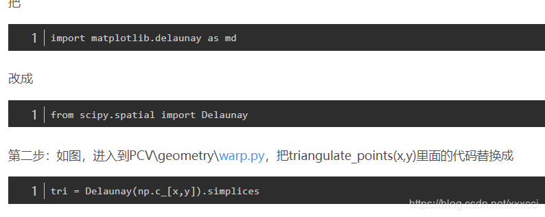
另外还有wrap.py文件的报错，具体解决如下：
进入wrappy文件：