基于CelebA数据集训练DCGAN生成人脸（附完整代码和解读）

ialover

已于 2024-11-29 14:32:56 修改

阅读量1.6k

点赞数 27

文章标签： python

于 2024-11-28 23:37:32 首次发布

本文链接：https://blog.csdn.net/yaoyihe/article/details/144122940

版权

在本篇博客中，我们将详细介绍如何使用DCGAN（生成对抗网络）来生成人脸图像。我们将使用CelebA数据集进行训练，分析网络结构、损失函数、优化器以及生成和判别器的工作原理，并提供完整的代码实现。最后，我们将展示如何通过训练得到的生成器生成合成的人脸图像。

GAN简介

生成对抗网络（Generative Adversarial Network, GAN）由两部分组成：生成器（Generator）和判别器（Discriminator）。生成器的目标是生成逼真的图像，而判别器的目标是区分真假图像。在训练过程中，生成器和判别器通过对抗训练互相促进，最终生成器能够生成极其逼真的图像。

本实验基于DCGAN（Generative Convolutional GAN）结构，这是一种通过卷积神经网络（CNN）和反卷积（Transpose Convolution）网络来生成高质量图像的方法。

数据集介绍

本实验使用的是CelebA数据集，该数据集包含了大量的人脸图像，非常适合用于人脸生成的任务。数据集可以通过此链接下载。

代码解读

下面将分步解释代码的主要部分。

1. 导入必要的库

import argparse
import os
import random
import torch
import torch.nn as nn
import torch.nn.parallel
import torch.optim as optim
import torch.utils.data
import torchvision.datasets as dset
import torchvision.transforms as transforms
import torchvision.utils as vutils
import numpy as np
import matplotlib.pyplot as plt
import matplotlib.animation as animation
from IPython.display import HTML
import torchvision
from sympy.physics.units import dalton
from tqdm import tqdm
import time
import datetime

# 并行
import torch.nn.parallel
torch.use_deterministic_algorithms(True)

# 设置随机种子，使得代码结果可以复现
seed = 999
random.seed(seed)
torch.manual_seed(seed)
print(f"seed is {seed}")

首先，我们导入了深度学习所需的主要库，包括torch和torchvision，并且还引入了其他用于数据处理和可视化的库。

2. 设置训练参数

root_dir = 'document/gcgan'
worker = 4
image_size = 64
num_epochs = 50
batch_size = 128 
nc = 3  # 输入图片的通道数
nz = 100  # 生成器的输入潜在向量的维度
ngf = 64  # 生成器中卷积层的滤波器数量
ndf = 64  # 判别器中卷积层的滤波器数量
lr = 0.0002  # 优化器的学习率
beta1 = 0.5  # Adam优化器中的beta1超参数
ngpu = 1  # GPU的数量

我们设置了训练所需的各类超参数。image_size决定了输入图像的尺寸，batch_size表示每次训练输入的样本数量，nz是生成器的输入潜在空间维度，ngf和ndf分别表示生成器和判别器中卷积层的滤波器数量。

3. 数据预处理和加载

transform = transforms.Compose([
    transforms.Resize(image_size),
    transforms.CenterCrop(image_size),
    transforms.ToTensor(),
    transforms.Normalize((0.5, 0.5, 0.5), (0.5, 0.5, 0.5)),
])

dataset = torchvision.datasets.ImageFolder(root=root_dir, transform=transform)
dataloader = torch.utils.data.DataLoader(dataset, batch_size=batch_size, shuffle=True, num_workers=worker)

我们对CelebA数据集进行了预处理，包括调整图像大小、中心裁剪、转化为Tensor格式以及标准化。这些操作帮助我们将图像数据处理为训练时适用的格式。

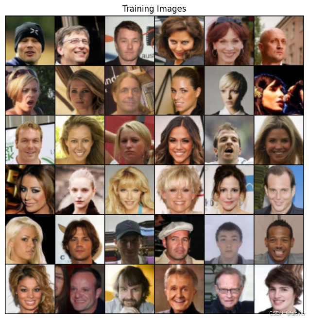
4. 数据的可视化

# 定义cuda or cpu 设备
device = 'cuda:0' if (torch.cuda.is_available() and ngpu >= 1) else 'cpu'
# 获得一批数据，并且可视化
real_batch = next(iter(dataloader)) #iter转化为迭代器，next获得一批数据
plt.figure(figsize = (8,8))
train_images = vutils.make_grid(real_batch[0].to(device)[:36],padding=1,normalize=True,nrow=6).cpu() #先获得一个批次中图像数据转入设备在提取需要的图像数
plt.imshow(np.transpose(train_images,(1,2,0)))
plt.axis('off')
plt.title('Training Images')
plt.show()

可视化结果

5. 网络结构

1.权重的初始化

def weights_init(m):
    classname = m.__class__.__name__ # 获得m模块的类名
    if classname.find('Conv') != -1:
        nn.init.normal_(m.weight.data, 0.0, 0.02)
    elif classname.find('BatchNorm') != -1:
        nn.init.normal_(m.weight.data, 1.0, 0.02)
        nn.init.constant_(m.bias.data, 0)

2.生成器（Generator）

生成器的任务是从随机噪声中生成图像。我们使用了一系列反卷积层来逐步扩展潜在向量的维度，并最终生成图像。

# 定义生成器网络
class Generator(nn.Module):
    def __init__(self,ngpu):
        super(Generator, self).__init__()
        self.ngpu = ngpu
        self.main = nn.Sequential(
            # 反卷积：输入是噪声的潜在维度，输出是ngf * 8
            nn.ConvTranspose2d(in_channels= nz, out_channels= ngf* 8, kernel_size=4,stride=1, padding=0, bias=False),
            # 归一化输出层
            nn.BatchNorm2d(ngf* 8),
            nn.ReLU(True),
            
            nn.ConvTranspose2d(ngf* 8, ngf* 4, kernel_size=4, stride=2, padding=1, bias=False),
            nn.BatchNorm2d(ngf* 4),
            nn.ReLU(True),
            
            nn.ConvTranspose2d(ngf* 4, ngf* 2, kernel_size=4, stride=2, padding=1, bias=False),
            nn.BatchNorm2d(ngf* 2),
            nn.ReLU(True),
            
            nn.ConvTranspose2d(ngf* 2, ngf, kernel_size=4, stride=2, padding=1, bias=False),
            nn.BatchNorm2d(ngf),
            nn.ReLU(True),
            
            nn.ConvTranspose2d(ngf, nc, kernel_size=4, stride=2, padding=1, bias=False),
            nn.Tanh()
        )
    def forward(self, input):
        return self.main(input)


# 初始化生成器和打印网络结构

netG = Generator(ngpu)
netG = netG.to(device)
if ngpu > 1 and device.type == 'cuda':
    netG = nn.DataParallel(netG, list(range(ngpu)))
netG.apply(weights_init)
print(netG)

输出

Generator(
  (main): Sequential(
    (0): ConvTranspose2d(100, 512, kernel_size=(4, 4), stride=(1, 1), bias=False)
    (1): BatchNorm2d(512, eps=1e-05, momentum=0.1, affine=True, track_running_stats=True)
    (2): ReLU(inplace=True)
    (3): ConvTranspose2d(512, 256, kernel_size=(4, 4), stride=(2, 2), padding=(1, 1), bias=False)
    (4): BatchNorm2d(256, eps=1e-05, momentum=0.1, affine=True, track_running_stats=True)
    (5): ReLU(inplace=True)
    (6): ConvTranspose2d(256, 128, kernel_size=(4, 4), stride=(2, 2), padding=(1, 1), bias=False)
    (7): BatchNorm2d(128, eps=1e-05, momentum=0.1, affine=True, track_running_stats=True)
    (8): ReLU(inplace=True)
    (9): ConvTranspose2d(128, 64, kernel_size=(4, 4), stride=(2, 2), padding=(1, 1), bias=False)
    (10): BatchNorm2d(64, eps=1e-05, momentum=0.1, affine=True, track_running_stats=True)
    (11): ReLU(inplace=True)
    (12): ConvTranspose2d(64, 3, kernel_size=(4, 4), stride=(2, 2), padding=(1, 1), bias=False)
    (13): Tanh()
  )
)

3.判别器（Discriminator）

判别器的任务是判断输入图像是真实的还是生成的。判别器由一系列卷积层构成，逐步缩小图像的尺寸，同时提取特征。


# 定义判别器网络结构
class Discriminator(nn.Module):
    def __init__(self,ngpu):
        super(Discriminator, self).__init__()
        self.ngpu = ngpu
        self.main = nn.Sequential(
            nn.Conv2d(nc, ndf, kernel_size=4, stride=2, padding=1, bias=False),
            nn.LeakyReLU(0.2, inplace=True),
            
            nn.Conv2d(ndf, ndf*2, kernel_size=4, stride=2, padding=1, bias=False),
            nn.BatchNorm2d(ndf*2),
            nn.LeakyReLU(0.2, inplace=True),
            
            nn.Conv2d(ndf*2, ndf*4, kernel_size=4, stride=2, padding=1, bias=False),
            nn.BatchNorm2d(ndf*4),
            nn.LeakyReLU(0.2, inplace=True),
            
            nn.Conv2d(ndf*4, ndf*8, kernel_size=4, stride=2, padding=1, bias=False),
            nn.BatchNorm2d(ndf*8),
            nn.LeakyReLU(0.2, inplace=True),
            
            nn.Conv2d(ndf*8, 1, kernel_size=4, stride=1, padding=0, bias=False),
            nn.Sigmoid()
        )
    def forward(self, input):
        return self.main(input)

# 初始化判别器和打印网络结构
netD = Discriminator(ngpu)
netD = netD.to(device)
if ngpu > 1 and device.type == 'cuda': 
    netD = nn.DataParallel(netD, list(range(ngpu)))
netD.apply(weights_init)
print(netD)

输出

Discriminator(
  (main): Sequential(
    (0): Conv2d(3, 64, kernel_size=(4, 4), stride=(2, 2), padding=(1, 1), bias=False)
    (1): LeakyReLU(negative_slope=0.2, inplace=True)
    (2): Conv2d(64, 128, kernel_size=(4, 4), stride=(2, 2), padding=(1, 1), bias=False)
    (3): BatchNorm2d(128, eps=1e-05, momentum=0.1, affine=True, track_running_stats=True)
    (4): LeakyReLU(negative_slope=0.2, inplace=True)
    (5): Conv2d(128, 256, kernel_size=(4, 4), stride=(2, 2), padding=(1, 1), bias=False)
    (6): BatchNorm2d(256, eps=1e-05, momentum=0.1, affine=True, track_running_stats=True)
    (7): LeakyReLU(negative_slope=0.2, inplace=True)
    (8): Conv2d(256, 512, kernel_size=(4, 4), stride=(2, 2), padding=(1, 1), bias=False)
    (9): BatchNorm2d(512, eps=1e-05, momentum=0.1, affine=True, track_running_stats=True)
    (10): LeakyReLU(negative_slope=0.2, inplace=True)
    (11): Conv2d(512, 1, kernel_size=(4, 4), stride=(1, 1), bias=False)
    (12): Sigmoid()
  )
)

6. 损失函数与优化器

我们使用二元交叉熵（BCELoss）作为损失函数，Adam优化器来更新网络参数。

criterion = nn.BCELoss()  # 二元交叉熵损失
real_label = 1.  # 真实标签
fake_label = 0.  # 假标签
optimizerD = optim.Adam(netD.parameters(), lr=lr, betas=(beta1, 0.999))
optimizerG = optim.Adam(netG.parameters(), lr=lr, betas=(beta1, 0.999))

7. 训练过程

在训练过程中，我们交替更新判别器和生成器。首先训练判别器，使其能够更好地区分真假图像，然后训练生成器，使其生成的假图像能够被判别器误认为是真实的。

# 生成器和判别器的训练
start_time = time.time()
print("Training Start :")
img_list  =[] #用于存储图像
G_losses = []
D_losses = []
iters = 0
for epoch in range(num_epochs):
    for i, data in enumerate(dataloader):
        # 训练代码
        # 训练判别器
        
        ############################
        # (1) Update D network: maximize log(D(x)) + log(1 - D(G(z)))
        ###########################
        
        # 训练判别器识别真图像
        netD.zero_grad()
        real_img = data[0].to(device) 
        img_num = real_img.size(0) # 获取图片的数量
        label = torch.full((img_num,),real_label,device=device,dtype= torch.float) # 创建真实类别标签
        output = netD(real_img).view(-1)
        D_real_loss = criterion(output,label)
        D_real_loss.backward()
        D_real_mean = output.mean().item() # 计算分类输出的平均值
        
        # 训练判别器识别假图像
        noise = torch.randn(img_num,nz,1,1,device = device)
        fake_img = netG(noise)
        label.fill_(fake_label) # 把 label 改为假图像的label
        output = netD(fake_img.detach()).view(-1) # detach() 是阻止梯度回到生成器
        D_fake_loss = criterion(output,label)
        D_fake_loss.backward()
        D_fake_mean = output.mean().item() 
        
        # 合并正确样本和错误样本的损失，更新判别器
        D_loss = D_real_loss + D_fake_loss
        optimizerD.step()
        
        
        ############################
        # (2) Update G network: maximize log(D(G(z)))
        ###########################
        
        # 训练生成器
        netG.zero_grad()
        label.fill_(real_label) # 就是要让判别器认为假图像是真图像
        output = netD(fake_img).view(-1)
        G_loss = criterion(output,label)
        G_loss.backward()
        G_mean = output.mean().item()
        optimizerG.step()
        
        # 输出损失和准确率
        if i % 100 == 0:
            print(f"[{epoch}/{num_epochs}][{i}/{len(dataloader)}]\t"
            f"Loss_D: {G_loss.item():.4f}\tLoss_G: {G_mean:.4f}\t"
            f"D(x): {D_real_mean:.4f},\tD(G(z)): {D_fake_mean:.4f} / {G_mean:.4f}")
        
        # 保存损失
        D_losses.append(D_loss.item())
        G_losses.append(G_loss.item())
        
        # 检测生成器的效果
        if (iters % 500 == 0) or ((epoch == num_epochs-1) and (i == len(dataloader)-1)):
            with torch.no_grad():
                fake_img = netG(fixed_noise).detach().cpu()
            img_list.append(vutils.make_grid(fake_img, padding=2, normalize=True,nrow=6).cpu())              
        iters += 1    

end_time = time.time()
total_time = end_time - start_time
formatted_time = str(datetime.timedelta(seconds=total_time))
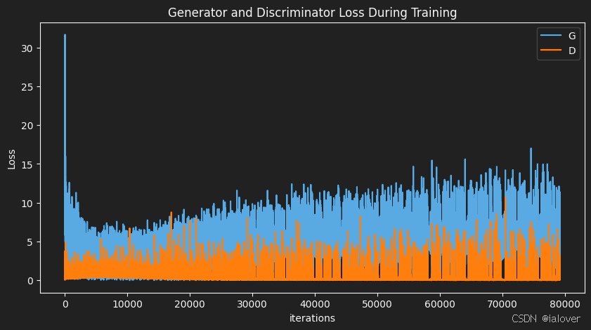
print(f"Total Training Time: {formatted_time}")

8. 训练结果展示

每隔一定的步数，我们会保存生成的图像并绘制损失曲线：

plt.figure(figsize=(10,5))
plt.title("Generator and Discriminator Loss During Training")
plt.plot(G_losses,label="G")
plt.plot(D_losses,label="D")
plt.xlabel("iterations")
plt.ylabel("Loss")
plt.legend()
plt.show()

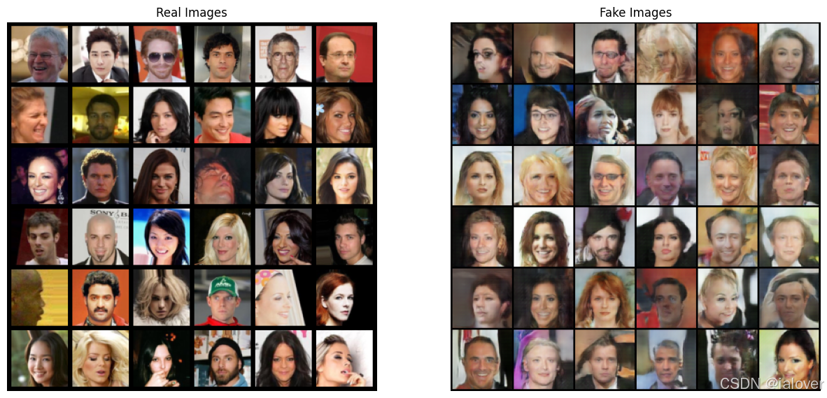
real_batch = next(iter(dataloader))
fig,axi = plt.subplots(1,2,figsize = (15,15))
axi = axi.flatten()
real_images = vutils.make_grid(real_batch[0].to(device)[:36],padding = 5,nrow=6,normalize=True).cpu()
axi[0].imshow(np.transpose(real_images,(1,2,0)))
axi[0].axis("off")
axi[0].set_title("Real Images")

axi[1].imshow(np.transpose(img_list[-1],(1,2,0)))
axi[1].axis("off")
axi[1].set_title("Fake Images")
plt.show()

输出

完整代码（复制可以直接运行）

import argparse
import os
import random
import torch
import torch.nn as nn
import torch.nn.parallel
import torch.optim as optim
import torch.utils.data
import torchvision.datasets as dset
import torchvision.transforms as transforms
import torchvision.utils as vutils
import numpy as np
import matplotlib.pyplot as plt
import matplotlib.animation as animation
from IPython.display import HTML
import torchvision
from sympy.physics.units import dalton
from tqdm import tqdm
import time
import datetime

# 并行
import torch.nn.parallel
torch.use_deterministic_algorithms(True)

# 设置随机种子，使得代码结果可以复现
seed = 999
random.seed(seed)
torch.manual_seed(seed)
print(f"seed is {seed}")


# 定义参数和数据集路径
root_dir = 'document/gcgan'

worker = 4
image_size = 64
num_epochs = 50
batch_size = 128 # 是批次大小，指的是一次输入的样本数
nc =3 # 输入图片的通道数
nz =100 # 生成器的输入潜在向量的维度
ngf = 64 # 生成器中卷积层的滤波器数量
ndf = 64 # 判别器中卷积层的滤波器数量
lr = 0.0002 # 优化器的学习率
beta1 = 0.5 # beta1 是 Adam 优化器中的 beta1 超参数
ngpu = 1 # GPU的数量，默认是1


# 导入数据集 和数据预处理
transform = transforms.Compose(
    [
        transforms.Resize(image_size),
        transforms.CenterCrop(image_size),
        transforms.ToTensor(),
        transforms.Normalize((0.5, 0.5, 0.5), (0.5, 0.5, 0.5)),
    ]
)
dataset = torchvision.datasets.ImageFolder(root = root_dir,transform= transform)
dataloader = torch.utils.data.DataLoader(dataset, batch_size = batch_size, shuffle = True,num_workers = worker)
# 定义cuda or cpu 设备
device = 'cuda:0' if (torch.cuda.is_available() and ngpu >= 1) else 'cpu'
# 获得一批数据，并且可视化
real_batch = next(iter(dataloader)) #iter转化为迭代器，next获得一批数据
plt.figure(figsize = (8,8))
train_images = vutils.make_grid(real_batch[0].to(device)[:36],padding=1,normalize=True,nrow=6).cpu() #先获得一个批次中图像数据转入设备在提取需要的图像数
plt.imshow(np.transpose(train_images,(1,2,0)))
plt.axis('off')
plt.title('Training Images')
plt.show()


def weights_init(m):
    classname = m.__class__.__name__ # 获得m模块的类名
    if classname.find('Conv') != -1:
        nn.init.normal_(m.weight.data, 0.0, 0.02)
    elif classname.find('BatchNorm') != -1:
        nn.init.normal_(m.weight.data, 1.0, 0.02)
        nn.init.constant_(m.bias.data, 0)


# 定义生成器网络
class Generator(nn.Module):
    def __init__(self,ngpu):
        super(Generator, self).__init__()
        self.ngpu = ngpu
        self.main = nn.Sequential(
            # 反卷积：输入是噪声的潜在维度，输出是ngf * 8
            nn.ConvTranspose2d(in_channels= nz, out_channels= ngf* 8, kernel_size=4,stride=1, padding=0, bias=False),
            # 归一化输出层
            nn.BatchNorm2d(ngf* 8),
            nn.ReLU(True),
            
            nn.ConvTranspose2d(ngf* 8, ngf* 4, kernel_size=4, stride=2, padding=1, bias=False),
            nn.BatchNorm2d(ngf* 4),
            nn.ReLU(True),
            
            nn.ConvTranspose2d(ngf* 4, ngf* 2, kernel_size=4, stride=2, padding=1, bias=False),
            nn.BatchNorm2d(ngf* 2),
            nn.ReLU(True),
            
            nn.ConvTranspose2d(ngf* 2, ngf, kernel_size=4, stride=2, padding=1, bias=False),
            nn.BatchNorm2d(ngf),
            nn.ReLU(True),
            
            nn.ConvTranspose2d(ngf, nc, kernel_size=4, stride=2, padding=1, bias=False),
            nn.Tanh()
        )
    def forward(self, input):
        return self.main(input)
        


# 初始化生成器和打印网络结构

netG = Generator(ngpu)
netG = netG.to(device)
if ngpu > 1 and device.type == 'cuda':
    netG = nn.DataParallel(netG, list(range(ngpu)))
netG.apply(weights_init)
print(netG)
    



# 定义判别器网络结构
class Discriminator(nn.Module):
    def __init__(self,ngpu):
        super(Discriminator, self).__init__()
        self.ngpu = ngpu
        self.main = nn.Sequential(
            nn.Conv2d(nc, ndf, kernel_size=4, stride=2, padding=1, bias=False),
            nn.LeakyReLU(0.2, inplace=True),
            
            nn.Conv2d(ndf, ndf*2, kernel_size=4, stride=2, padding=1, bias=False),
            nn.BatchNorm2d(ndf*2),
            nn.LeakyReLU(0.2, inplace=True),
            
            nn.Conv2d(ndf*2, ndf*4, kernel_size=4, stride=2, padding=1, bias=False),
            nn.BatchNorm2d(ndf*4),
            nn.LeakyReLU(0.2, inplace=True),
            
            nn.Conv2d(ndf*4, ndf*8, kernel_size=4, stride=2, padding=1, bias=False),
            nn.BatchNorm2d(ndf*8),
            nn.LeakyReLU(0.2, inplace=True),
            
            nn.Conv2d(ndf*8, 1, kernel_size=4, stride=1, padding=0, bias=False),
            nn.Sigmoid()
        )
    def forward(self, input):
        return self.main(input)
    


# 初始化判别器和打印网络结构
netD = Discriminator(ngpu)
netD = netD.to(device)
if ngpu > 1 and device.type == 'cuda': 
    netD = nn.DataParallel(netD, list(range(ngpu)))
netD.apply(weights_init)
print(netD)


# 定义损失函数和优化器
criterion = nn.BCELoss() # 使用二元交叉熵损失函数
real_label = 1.
fake_label = 0.
optimizerD = optim.Adam(netD.parameters(),lr = lr, betas = (beta1, 0.999))
optimizerG = optim.Adam(netG.parameters(),lr = lr, betas = (beta1, 0.999))
# 生成随机噪声
fixed_noise = torch.randn(36,nz,1,1,device=device) #主要用于后面的可视化


# 生成器和判别器的训练
start_time = time.time()
print("Training Start :")
img_list  =[] #用于存储图像
G_losses = []
D_losses = []
iters = 0
for epoch in range(num_epochs):
    # 包装 dataloader 的 enumerate，添加进度条
    for i, data in enumerate(dataloader):
        # 训练代码
        # 训练判别器
        
        ############################
        # (1) Update D network: maximize log(D(x)) + log(1 - D(G(z)))
        ###########################
        
        # 训练判别器识别真图像
        netD.zero_grad()
        real_img = data[0].to(device) 
        img_num = real_img.size(0) # 获取图片的数量
        label = torch.full((img_num,),real_label,device=device,dtype= torch.float) # 创建真实类别标签
        output = netD(real_img).view(-1)
        D_real_loss = criterion(output,label)
        D_real_loss.backward()
        D_real_mean = output.mean().item() # 计算分类输出的平均值
        
        # 训练判别器识别假图像
        noise = torch.randn(img_num,nz,1,1,device = device)
        fake_img = netG(noise)
        label.fill_(fake_label) # 把 label 改为假图像的label
        output = netD(fake_img.detach()).view(-1) # detach() 是阻止梯度回到生成器
        D_fake_loss = criterion(output,label)
        D_fake_loss.backward()
        D_fake_mean = output.mean().item() 
        
        # 合并正确样本和错误样本的损失，更新判别器
        D_loss = D_real_loss + D_fake_loss
        optimizerD.step()
        
        
        ############################
        # (2) Update G network: maximize log(D(G(z)))
        ###########################
        
        # 训练生成器
        netG.zero_grad()
        label.fill_(real_label) # 就是要让判别器认为假图像是真图像
        output = netD(fake_img).view(-1)
        G_loss = criterion(output,label)
        G_loss.backward()
        G_mean = output.mean().item()
        optimizerG.step()
        
        # 输出损失和准确率
        if i % 100 == 0:
            print(f"[{epoch}/{num_epochs}][{i}/{len(dataloader)}]\t"
            f"Loss_D: {G_loss.item():.4f}\tLoss_G: {G_mean:.4f}\t"
            f"D(x): {D_real_mean:.4f},\tD(G(z)): {D_fake_mean:.4f} / {G_mean:.4f}")
        
        # 保存损失
        D_losses.append(D_loss.item())
        G_losses.append(G_loss.item())
        
        # 检测生成器的效果
        if (iters % 500 == 0) or ((epoch == num_epochs-1) and (i == len(dataloader)-1)):
            with torch.no_grad():
                fake_img = netG(fixed_noise).detach().cpu()
            img_list.append(vutils.make_grid(fake_img, padding=2, normalize=True,nrow=6).cpu())              
        iters += 1    

end_time = time.time()
total_time = end_time - start_time
formatted_time = str(datetime.timedelta(seconds=total_time))
print(f"Total Training Time: {formatted_time}")

plt.figure(figsize=(10,5))
plt.title("Generator and Discriminator Loss During Training")
plt.plot(G_losses,label="G")
plt.plot(D_losses,label="D")
plt.xlabel("iterations")
plt.ylabel("Loss")
plt.legend()
plt.show()

real_batch = next(iter(dataloader))
fig,axi = plt.subplots(1,2,figsize = (15,15))
axi = axi.flatten()
real_images = vutils.make_grid(real_batch[0].to(device)[:36],padding = 5,nrow=6,normalize=True).cpu()
axi[0].imshow(np.transpose(real_images,(1,2,0)))
axi[0].axis("off")
axi[0].set_title("Real Images")

axi[1].imshow(np.transpose(img_list[-1],(1,2,0)))
axi[1].axis("off")
axi[1].set_title("Fake Images")
plt.show()