本文是对pandas的一个入门介绍,仅仅针对初学者。如果需要更详细的内容,请移步[Cookbook](http://pandas.pydata.org/pandas-docs/stable/cookbook.html#cookbook). 首先,导入所需要的python包:
import pandas as pd
import numpy as np
import matplotlib.pyplot as plt
创建对象 ———– pandas中的数据结构包括Series、DataFrame、Panel、Pannel4D等,详细介绍移步[数据结构介绍](http://pandas.pydata.org/pandas-docs/stable/dsintro.html#dsintro). 常用的数据结构是前两个:Series和DataFrame。 通过传入一个已有的python列表(list)对象来创建一个Series对象。
s = pd.Series([1,3,4,np.nan,6,8])
s
0 1.0 1 3.0 2 4.0 3 NaN 4 6.0 5 8.0 dtype: float64 通过传入一个numpy数组来构建一个DataFrame对象。使用时间序列作为每行的索引,并为每列数据分配一个列名。
dates = pd.date_range('20130101', periods=6)
dates
DatetimeIndex([‘2013-01-01’, ‘2013-01-02’, ‘2013-01-03’, ‘2013-01-04’, ‘2013-01-05’, ‘2013-01-06’], dtype=’datetime64[ns]’, freq=’D’)
df = pd.DataFrame(np.random.randn(6,4), index=dates, columns=list('ABCD'))
df
| A | B | C | D |
|---|
| 2013-01-01 | -0.285894 | 0.490011 | 0.171121 | -1.549807 |
|---|
| 2013-01-02 | -0.068377 | -0.452804 | -0.391892 | -0.852520 |
|---|
| 2013-01-03 | 1.304388 | -1.808484 | -0.286489 | -0.437457 |
|---|
| 2013-01-04 | 1.447812 | -1.862121 | 0.115950 | -0.664134 |
|---|
| 2013-01-05 | 0.520409 | -1.402740 | -0.356049 | 0.460950 |
|---|
| 2013-01-06 | -0.404900 | 0.585420 | -0.073923 | -0.501197 |
|---|
通过传入一个python字典对象来创建一个DataFrame对象。
df2 = pd.DataFrame({'A': 1.,
                    'B': pd.Timestamp('20160102'),
                    'C': pd.Series(1,index=list(range(4)),dtype='float32'),
                    'D': np.array([3]*4, dtype='int32'),
                    'E': pd.Categorical(['test','train','test','train']),
                    'F': 'foo'})
df2
| A | B | C | D | E | F |
|---|
| 0 | 1.0 | 2016-01-02 | 1.0 | 3 | test | foo |
|---|
| 1 | 1.0 | 2016-01-02 | 1.0 | 3 | train | foo |
|---|
| 2 | 1.0 | 2016-01-02 | 1.0 | 3 | test | foo |
|---|
| 3 | 1.0 | 2016-01-02 | 1.0 | 3 | train | foo |
|---|
df2.dtypes
A           float64
B    datetime64[ns]
C           float32
D             int32
E          category
F            object
dtype: object
在ipython中可以使用“Tab”键对DataFrame的列名和公共属性进行自动补全。
查看对象中的数据
查看DataFrame的前几行或最后几行
df.head()
| A | B | C | D |
|---|
| 2013-01-01 | -0.285894 | 0.490011 | 0.171121 | -1.549807 |
|---|
| 2013-01-02 | -0.068377 | -0.452804 | -0.391892 | -0.852520 |
|---|
| 2013-01-03 | 1.304388 | -1.808484 | -0.286489 | -0.437457 |
|---|
| 2013-01-04 | 1.447812 | -1.862121 | 0.115950 | -0.664134 |
|---|
| 2013-01-05 | 0.520409 | -1.402740 | -0.356049 | 0.460950 |
|---|
df.tail()
| A | B | C | D |
|---|
| 2013-01-02 | -0.068377 | -0.452804 | -0.391892 | -0.852520 |
|---|
| 2013-01-03 | 1.304388 | -1.808484 | -0.286489 | -0.437457 |
|---|
| 2013-01-04 | 1.447812 | -1.862121 | 0.115950 | -0.664134 |
|---|
| 2013-01-05 | 0.520409 | -1.402740 | -0.356049 | 0.460950 |
|---|
| 2013-01-06 | -0.404900 | 0.585420 | -0.073923 | -0.501197 |
|---|
df.head(3)
| A | B | C | D |
|---|
| 2013-01-01 | -0.285894 | 0.490011 | 0.171121 | -1.549807 |
|---|
| 2013-01-02 | -0.068377 | -0.452804 | -0.391892 | -0.852520 |
|---|
| 2013-01-03 | 1.304388 | -1.808484 | -0.286489 | -0.437457 |
|---|
获取DataFrame的索引、列名、数据(值)。
df.index
DatetimeIndex(['2013-01-01', '2013-01-02', '2013-01-03', '2013-01-04',
               '2013-01-05', '2013-01-06'],
              dtype='datetime64[ns]', freq='D')
df.columns
Index([u'A', u'B', u'C', u'D'], dtype='object')
df.values
array([[-0.28589413,  0.49001051,  0.17112101, -1.54980655],
       [-0.06837701, -0.45280422, -0.39189213, -0.85252018],
       [ 1.30438846, -1.80848416, -0.28648908, -0.43745725],
       [ 1.44781215, -1.86212061,  0.11594994, -0.66413402],
       [ 0.5204089 , -1.4027399 , -0.35604882,  0.4609499 ],
       [-0.40489995,  0.58541997, -0.07392295, -0.5011969 ]])
使用“describe”获取数据的统计信息。
df.describe()
| A | B | C | D |
|---|
| count | 6.000000 | 6.000000 | 6.000000 | 6.000000 |
|---|
| mean | 0.418906 | -0.741786 | -0.136880 | -0.590694 |
|---|
| std | 0.808192 | 1.112849 | 0.244213 | 0.652884 |
|---|
| min | -0.404900 | -1.862121 | -0.391892 | -1.549807 |
|---|
| 25% | -0.231515 | -1.707048 | -0.338659 | -0.805424 |
|---|
| 50% | 0.226016 | -0.927772 | -0.180206 | -0.582665 |
|---|
| 75% | 1.108394 | 0.254307 | 0.068482 | -0.453392 |
|---|
| max | 1.447812 | 0.585420 | 0.171121 | 0.460950 |
|---|
将DataFrame进行转置。
df.T
| 2013-01-01 00:00:00 | 2013-01-02 00:00:00 | 2013-01-03 00:00:00 | 2013-01-04 00:00:00 | 2013-01-05 00:00:00 | 2013-01-06 00:00:00 |
|---|
| A | -0.285894 | -0.068377 | 1.304388 | 1.447812 | 0.520409 | -0.404900 |
|---|
| B | 0.490011 | -0.452804 | -1.808484 | -1.862121 | -1.402740 | 0.585420 |
|---|
| C | 0.171121 | -0.391892 | -0.286489 | 0.115950 | -0.356049 | -0.073923 |
|---|
| D | -1.549807 | -0.852520 | -0.437457 | -0.664134 | 0.460950 | -0.501197 |
|---|
df
| A | B | C | D |
|---|
| 2013-01-01 | -0.285894 | 0.490011 | 0.171121 | -1.549807 |
|---|
| 2013-01-02 | -0.068377 | -0.452804 | -0.391892 | -0.852520 |
|---|
| 2013-01-03 | 1.304388 | -1.808484 | -0.286489 | -0.437457 |
|---|
| 2013-01-04 | 1.447812 | -1.862121 | 0.115950 | -0.664134 |
|---|
| 2013-01-05 | 0.520409 | -1.402740 | -0.356049 | 0.460950 |
|---|
| 2013-01-06 | -0.404900 | 0.585420 | -0.073923 | -0.501197 |
|---|
对坐标轴进行排序。
df.sort_index(axis=1, ascending=False)
| D | C | B | A |
|---|
| 2013-01-01 | -1.549807 | 0.171121 | 0.490011 | -0.285894 |
|---|
| 2013-01-02 | -0.852520 | -0.391892 | -0.452804 | -0.068377 |
|---|
| 2013-01-03 | -0.437457 | -0.286489 | -1.808484 | 1.304388 |
|---|
| 2013-01-04 | -0.664134 | 0.115950 | -1.862121 | 1.447812 |
|---|
| 2013-01-05 | 0.460950 | -0.356049 | -1.402740 | 0.520409 |
|---|
| 2013-01-06 | -0.501197 | -0.073923 | 0.585420 | -0.404900 |
|---|
df.sort_index(axis=0, ascending=False)
| A | B | C | D |
|---|
| 2013-01-06 | -0.404900 | 0.585420 | -0.073923 | -0.501197 |
|---|
| 2013-01-05 | 0.520409 | -1.402740 | -0.356049 | 0.460950 |
|---|
| 2013-01-04 | 1.447812 | -1.862121 | 0.115950 | -0.664134 |
|---|
| 2013-01-03 | 1.304388 | -1.808484 | -0.286489 | -0.437457 |
|---|
| 2013-01-02 | -0.068377 | -0.452804 | -0.391892 | -0.852520 |
|---|
| 2013-01-01 | -0.285894 | 0.490011 | 0.171121 | -1.549807 |
|---|
对值进行排序。
df.sort_values(by='B')
| A | B | C | D |
|---|
| 2013-01-04 | 1.447812 | -1.862121 | 0.115950 | -0.664134 |
|---|
| 2013-01-03 | 1.304388 | -1.808484 | -0.286489 | -0.437457 |
|---|
| 2013-01-05 | 0.520409 | -1.402740 | -0.356049 | 0.460950 |
|---|
| 2013-01-02 | -0.068377 | -0.452804 | -0.391892 | -0.852520 |
|---|
| 2013-01-01 | -0.285894 | 0.490011 | 0.171121 | -1.549807 |
|---|
| 2013-01-06 | -0.404900 | 0.585420 | -0.073923 | -0.501197 |
|---|
df.sort_values(by='B',ascending=False)
| A | B | C | D |
|---|
| 2013-01-06 | -0.404900 | 0.585420 | -0.073923 | -0.501197 |
|---|
| 2013-01-01 | -0.285894 | 0.490011 | 0.171121 | -1.549807 |
|---|
| 2013-01-02 | -0.068377 | -0.452804 | -0.391892 | -0.852520 |
|---|
| 2013-01-05 | 0.520409 | -1.402740 | -0.356049 | 0.460950 |
|---|
| 2013-01-03 | 1.304388 | -1.808484 | -0.286489 | -0.437457 |
|---|
| 2013-01-04 | 1.447812 | -1.862121 | 0.115950 | -0.664134 |
|---|
选择数据
pandas中对数据的选择可以使用标准的python/numpy方式。
df['A']
2013-01-01   -0.285894
2013-01-02   -0.068377
2013-01-03    1.304388
2013-01-04    1.447812
2013-01-05    0.520409
2013-01-06   -0.404900
Freq: D, Name: A, dtype: float64
df.A
2013-01-01   -0.285894
2013-01-02   -0.068377
2013-01-03    1.304388
2013-01-04    1.447812
2013-01-05    0.520409
2013-01-06   -0.404900
Freq: D, Name: A, dtype: float64
对行进行切片操作。
df[0:3]
| A | B | C | D |
|---|
| 2013-01-01 | -0.285894 | 0.490011 | 0.171121 | -1.549807 |
|---|
| 2013-01-02 | -0.068377 | -0.452804 | -0.391892 | -0.852520 |
|---|
| 2013-01-03 | 1.304388 | -1.808484 | -0.286489 | -0.437457 |
|---|
df['20130103':'20130105']
| A | B | C | D |
|---|
| 2013-01-03 | 1.304388 | -1.808484 | -0.286489 | -0.437457 |
|---|
| 2013-01-04 | 1.447812 | -1.862121 | 0.115950 | -0.664134 |
|---|
| 2013-01-05 | 0.520409 | -1.402740 | -0.356049 | 0.460950 |
|---|
使用标准的python/numpy方法获取数据的方式很直观,但是对于工业级的代码,建议使用优化的pandas数据获取方法,包括:.at,.iat,.iloc和.ix
df
| A | B | C | D |
|---|
| 2013-01-01 | -0.285894 | 0.490011 | 0.171121 | -1.549807 |
|---|
| 2013-01-02 | -0.068377 | -0.452804 | -0.391892 | -0.852520 |
|---|
| 2013-01-03 | 1.304388 | -1.808484 | -0.286489 | -0.437457 |
|---|
| 2013-01-04 | 1.447812 | -1.862121 | 0.115950 | -0.664134 |
|---|
| 2013-01-05 | 0.520409 | -1.402740 | -0.356049 | 0.460950 |
|---|
| 2013-01-06 | -0.404900 | 0.585420 | -0.073923 | -0.501197 |
|---|
dates
DatetimeIndex(['2013-01-01', '2013-01-02', '2013-01-03', '2013-01-04',
               '2013-01-05', '2013-01-06'],
              dtype='datetime64[ns]', freq='D')
df.loc[dates[0]]
A   -0.285894
B    0.490011
C    0.171121
D   -1.549807
Name: 2013-01-01 00:00:00, dtype: float64
按类标选择多坐标轴的数据。
df.loc[:,['A','B']]
| A | B |
|---|
| 2013-01-01 | -0.285894 | 0.490011 |
|---|
| 2013-01-02 | -0.068377 | -0.452804 |
|---|
| 2013-01-03 | 1.304388 | -1.808484 |
|---|
| 2013-01-04 | 1.447812 | -1.862121 |
|---|
| 2013-01-05 | 0.520409 | -1.402740 |
|---|
| 2013-01-06 | -0.404900 | 0.585420 |
|---|
df.loc['20130102':'20130104',['A','B']]
| A | B |
|---|
| 2013-01-02 | -0.068377 | -0.452804 |
|---|
| 2013-01-03 | 1.304388 | -1.808484 |
|---|
| 2013-01-04 | 1.447812 | -1.862121 |
|---|
df.loc['20130105',['A','B']]
A    0.520409
B   -1.402740
Name: 2013-01-05 00:00:00, dtype: float64
df.loc['20130105','A']
0.52040890430486719
df.at[dates[0],'A']
-0.28589413005579967
按位置进行选择,传入整数,返回数据。
df
| A | B | C | D |
|---|
| 2013-01-01 | -0.285894 | 0.490011 | 0.171121 | -1.549807 |
|---|
| 2013-01-02 | -0.068377 | -0.452804 | -0.391892 | -0.852520 |
|---|
| 2013-01-03 | 1.304388 | -1.808484 | -0.286489 | -0.437457 |
|---|
| 2013-01-04 | 1.447812 | -1.862121 | 0.115950 | -0.664134 |
|---|
| 2013-01-05 | 0.520409 | -1.402740 | -0.356049 | 0.460950 |
|---|
| 2013-01-06 | -0.404900 | 0.585420 | -0.073923 | -0.501197 |
|---|
df.iloc[3]
A    1.447812
B   -1.862121
C    0.115950
D   -0.664134
Name: 2013-01-04 00:00:00, dtype: float64
df.iloc[3:5,0:2]
| A | B |
|---|
| 2013-01-04 | 1.447812 | -1.862121 |
|---|
| 2013-01-05 | 0.520409 | -1.402740 |
|---|
按整数位置进行数据选取或切片时,方法同python/numpy,从0开始索引,包含前端不含后端。
df.iloc[[1,2,4],[0,2]]
| A | C |
|---|
| 2013-01-02 | -0.068377 | -0.391892 |
|---|
| 2013-01-03 | 1.304388 | -0.286489 |
|---|
| 2013-01-05 | 0.520409 | -0.356049 |
|---|
df.iloc[1:3,:]
| A | B | C | D |
|---|
| 2013-01-02 | -0.068377 | -0.452804 | -0.391892 | -0.852520 |
|---|
| 2013-01-03 | 1.304388 | -1.808484 | -0.286489 | -0.437457 |
|---|
df.iloc[:,1:3]
| B | C |
|---|
| 2013-01-01 | 0.490011 | 0.171121 |
|---|
| 2013-01-02 | -0.452804 | -0.391892 |
|---|
| 2013-01-03 | -1.808484 | -0.286489 |
|---|
| 2013-01-04 | -1.862121 | 0.115950 |
|---|
| 2013-01-05 | -1.402740 | -0.356049 |
|---|
| 2013-01-06 | 0.585420 | -0.073923 |
|---|
df.iloc[1,1]
-0.45280421688689004
df.iat[1,1]
-0.45280421688689004
使用布尔值进行索引。
df[df.A > 0]
| A | B | C | D |
|---|
| 2013-01-03 | 1.304388 | -1.808484 | -0.286489 | -0.437457 |
|---|
| 2013-01-04 | 1.447812 | -1.862121 | 0.115950 | -0.664134 |
|---|
| 2013-01-05 | 0.520409 | -1.402740 | -0.356049 | 0.460950 |
|---|
df[df > 0]
| A | B | C | D |
|---|
| 2013-01-01 | NaN | 0.490011 | 0.171121 | NaN |
|---|
| 2013-01-02 | NaN | NaN | NaN | NaN |
|---|
| 2013-01-03 | 1.304388 | NaN | NaN | NaN |
|---|
| 2013-01-04 | 1.447812 | NaN | 0.115950 | NaN |
|---|
| 2013-01-05 | 0.520409 | NaN | NaN | 0.46095 |
|---|
| 2013-01-06 | NaN | 0.585420 | NaN | NaN |
|---|
使用isin()方法进行过滤。
df2 = df.copy()
df2['E'] = ['one','one','two','three','four','three']
df2
| A | B | C | D | E |
|---|
| 2013-01-01 | -0.285894 | 0.490011 | 0.171121 | -1.549807 | one |
|---|
| 2013-01-02 | -0.068377 | -0.452804 | -0.391892 | -0.852520 | one |
|---|
| 2013-01-03 | 1.304388 | -1.808484 | -0.286489 | -0.437457 | two |
|---|
| 2013-01-04 | 1.447812 | -1.862121 | 0.115950 | -0.664134 | three |
|---|
| 2013-01-05 | 0.520409 | -1.402740 | -0.356049 | 0.460950 | four |
|---|
| 2013-01-06 | -0.404900 | 0.585420 | -0.073923 | -0.501197 | three |
|---|
df2[df2['E'].isin(['one','four'])]
| A | B | C | D | E |
|---|
| 2013-01-01 | -0.285894 | 0.490011 | 0.171121 | -1.549807 | one |
|---|
| 2013-01-02 | -0.068377 | -0.452804 | -0.391892 | -0.852520 | one |
|---|
| 2013-01-05 | 0.520409 | -1.402740 | -0.356049 | 0.460950 | four |
|---|
设置数据
设置一个新列,自动按索引分配数据。
s1 = pd.Series([1,2,3,4,5,6], index=pd.date_range('20130102',periods=6))
s1
2013-01-02    1
2013-01-03    2
2013-01-04    3
2013-01-05    4
2013-01-06    5
2013-01-07    6
Freq: D, dtype: int64
df['F'] = s1
df
| A | B | C | D | F |
|---|
| 2013-01-01 | -0.285894 | 0.490011 | 0.171121 | -1.549807 | NaN |
|---|
| 2013-01-02 | -0.068377 | -0.452804 | -0.391892 | -0.852520 | 1.0 |
|---|
| 2013-01-03 | 1.304388 | -1.808484 | -0.286489 | -0.437457 | 2.0 |
|---|
| 2013-01-04 | 1.447812 | -1.862121 | 0.115950 | -0.664134 | 3.0 |
|---|
| 2013-01-05 | 0.520409 | -1.402740 | -0.356049 | 0.460950 | 4.0 |
|---|
| 2013-01-06 | -0.404900 | 0.585420 | -0.073923 | -0.501197 | 5.0 |
|---|
因为s1是从‘20130102’开始的,所以‘20130101’对应的F列值为‘NaN’
df.at[dates[0],'A'] = 0
df
| A | B | C | D | F |
|---|
| 2013-01-01 | 0.000000 | 0.490011 | 0.171121 | -1.549807 | NaN |
|---|
| 2013-01-02 | -0.068377 | -0.452804 | -0.391892 | -0.852520 | 1.0 |
|---|
| 2013-01-03 | 1.304388 | -1.808484 | -0.286489 | -0.437457 | 2.0 |
|---|
| 2013-01-04 | 1.447812 | -1.862121 | 0.115950 | -0.664134 | 3.0 |
|---|
| 2013-01-05 | 0.520409 | -1.402740 | -0.356049 | 0.460950 | 4.0 |
|---|
| 2013-01-06 | -0.404900 | 0.585420 | -0.073923 | -0.501197 | 5.0 |
|---|
df.iat[0,1] = 0
df.loc[:,'D'] = np.array([5] * len(df))
df
| A | B | C | D | F |
|---|
| 2013-01-01 | 0.000000 | 0.000000 | 0.171121 | 5 | NaN |
|---|
| 2013-01-02 | -0.068377 | -0.452804 | -0.391892 | 5 | 1.0 |
|---|
| 2013-01-03 | 1.304388 | -1.808484 | -0.286489 | 5 | 2.0 |
|---|
| 2013-01-04 | 1.447812 | -1.862121 | 0.115950 | 5 | 3.0 |
|---|
| 2013-01-05 | 0.520409 | -1.402740 | -0.356049 | 5 | 4.0 |
|---|
| 2013-01-06 | -0.404900 | 0.585420 | -0.073923 | 5 | 5.0 |
|---|
df2 = df.copy()
df2[df2 > 0] = -df2
df2
| A | B | C | D | F |
|---|
| 2013-01-01 | 0.000000 | 0.000000 | -0.171121 | -5 | NaN |
|---|
| 2013-01-02 | -0.068377 | -0.452804 | -0.391892 | -5 | -1.0 |
|---|
| 2013-01-03 | -1.304388 | -1.808484 | -0.286489 | -5 | -2.0 |
|---|
| 2013-01-04 | -1.447812 | -1.862121 | -0.115950 | -5 | -3.0 |
|---|
| 2013-01-05 | -0.520409 | -1.402740 | -0.356049 | -5 | -4.0 |
|---|
| 2013-01-06 | -0.404900 | -0.585420 | -0.073923 | -5 | -5.0 |
|---|
缺失数据
pandas主要使用”np.nan“表示缺失数据,默认是不参与计算的。
“reindex”使我们可以对某个轴上的索引进行增删改操作。这种操作返回的是数据的一个备份。
df1 = df.reindex(index=dates[0:4], columns=list(df.columns)+['E'])
df1.loc[dates[0]:dates[1],'E'] = 1
df1
| A | B | C | D | F | E |
|---|
| 2013-01-01 | 0.000000 | 0.000000 | 0.171121 | 5 | NaN | 1.0 |
|---|
| 2013-01-02 | -0.068377 | -0.452804 | -0.391892 | 5 | 1.0 | 1.0 |
|---|
| 2013-01-03 | 1.304388 | -1.808484 | -0.286489 | 5 | 2.0 | NaN |
|---|
| 2013-01-04 | 1.447812 | -1.862121 | 0.115950 | 5 | 3.0 | NaN |
|---|
df1.dropna(how='any')
| A | B | C | D | F | E |
|---|
| 2013-01-02 | -0.068377 | -0.452804 | -0.391892 | 5 | 1.0 | 1.0 |
|---|
df1.fillna(value=5)
| A | B | C | D | F | E |
|---|
| 2013-01-01 | 0.000000 | 0.000000 | 0.171121 | 5 | 5.0 | 1.0 |
|---|
| 2013-01-02 | -0.068377 | -0.452804 | -0.391892 | 5 | 1.0 | 1.0 |
|---|
| 2013-01-03 | 1.304388 | -1.808484 | -0.286489 | 5 | 2.0 | 5.0 |
|---|
| 2013-01-04 | 1.447812 | -1.862121 | 0.115950 | 5 | 3.0 | 5.0 |
|---|
pd.isnull(df1)
| A | B | C | D | F | E |
|---|
| 2013-01-01 | False | False | False | False | True | False |
|---|
| 2013-01-02 | False | False | False | False | False | False |
|---|
| 2013-01-03 | False | False | False | False | False | True |
|---|
| 2013-01-04 | False | False | False | False | False | True |
|---|
df1
| A | B | C | D | F | E |
|---|
| 2013-01-01 | 0.000000 | 0.000000 | 0.171121 | 5 | NaN | 1.0 |
|---|
| 2013-01-02 | -0.068377 | -0.452804 | -0.391892 | 5 | 1.0 | 1.0 |
|---|
| 2013-01-03 | 1.304388 | -1.808484 | -0.286489 | 5 | 2.0 | NaN |
|---|
| 2013-01-04 | 1.447812 | -1.862121 | 0.115950 | 5 | 3.0 | NaN |
|---|
运算
运算通常不含缺失值。
df
| A | B | C | D | F |
|---|
| 2013-01-01 | 0.000000 | 0.000000 | 0.171121 | 5 | NaN |
|---|
| 2013-01-02 | -0.068377 | -0.452804 | -0.391892 | 5 | 1.0 |
|---|
| 2013-01-03 | 1.304388 | -1.808484 | -0.286489 | 5 | 2.0 |
|---|
| 2013-01-04 | 1.447812 | -1.862121 | 0.115950 | 5 | 3.0 |
|---|
| 2013-01-05 | 0.520409 | -1.402740 | -0.356049 | 5 | 4.0 |
|---|
| 2013-01-06 | -0.404900 | 0.585420 | -0.073923 | 5 | 5.0 |
|---|
df.mean()
A    0.466555
B   -0.823455
C   -0.136880
D    5.000000
F    3.000000
dtype: float64
df.mean(1)
2013-01-01    1.292780
2013-01-02    1.017385
2013-01-03    1.241883
2013-01-04    1.540328
2013-01-05    1.552324
2013-01-06    2.021319
Freq: D, dtype: float64
在具有不同维度的对象之间进行运算时,需要进行对其。pandas会自动沿着特定维度进行扩展操作。
s = pd.Series([1,3,5,np.nan,6,8], index=dates)
s
2013-01-01    1.0
2013-01-02    3.0
2013-01-03    5.0
2013-01-04    NaN
2013-01-05    6.0
2013-01-06    8.0
Freq: D, dtype: float64
s = s.shift(2)
s
2013-01-01    NaN
2013-01-02    NaN
2013-01-03    1.0
2013-01-04    3.0
2013-01-05    5.0
2013-01-06    NaN
Freq: D, dtype: float64
df
| A | B | C | D | F |
|---|
| 2013-01-01 | 0.000000 | 0.000000 | 0.171121 | 5 | NaN |
|---|
| 2013-01-02 | -0.068377 | -0.452804 | -0.391892 | 5 | 1.0 |
|---|
| 2013-01-03 | 1.304388 | -1.808484 | -0.286489 | 5 | 2.0 |
|---|
| 2013-01-04 | 1.447812 | -1.862121 | 0.115950 | 5 | 3.0 |
|---|
| 2013-01-05 | 0.520409 | -1.402740 | -0.356049 | 5 | 4.0 |
|---|
| 2013-01-06 | -0.404900 | 0.585420 | -0.073923 | 5 | 5.0 |
|---|
df.sub(s,axis='index')
| A | B | C | D | F |
|---|
| 2013-01-01 | NaN | NaN | NaN | NaN | NaN |
|---|
| 2013-01-02 | NaN | NaN | NaN | NaN | NaN |
|---|
| 2013-01-03 | 0.304388 | -2.808484 | -1.286489 | 4.0 | 1.0 |
|---|
| 2013-01-04 | -1.552188 | -4.862121 | -2.884050 | 2.0 | 0.0 |
|---|
| 2013-01-05 | -4.479591 | -6.402740 | -5.356049 | 0.0 | -1.0 |
|---|
| 2013-01-06 | NaN | NaN | NaN | NaN | NaN |
|---|
sub()是减运算,df减去s时s的维度会自动进行扩展。
apply运算
apply运算将函数作用于数据。
df.apply(np.cumsum)
| A | B | C | D | F |
|---|
| 2013-01-01 | 0.000000 | 0.000000 | 0.171121 | 5 | NaN |
|---|
| 2013-01-02 | -0.068377 | -0.452804 | -0.220771 | 10 | 1.0 |
|---|
| 2013-01-03 | 1.236011 | -2.261288 | -0.507260 | 15 | 3.0 |
|---|
| 2013-01-04 | 2.683824 | -4.123409 | -0.391310 | 20 | 6.0 |
|---|
| 2013-01-05 | 3.204233 | -5.526149 | -0.747359 | 25 | 10.0 |
|---|
| 2013-01-06 | 2.799333 | -4.940729 | -0.821282 | 30 | 15.0 |
|---|
df
| A | B | C | D | F |
|---|
| 2013-01-01 | 0.000000 | 0.000000 | 0.171121 | 5 | NaN |
|---|
| 2013-01-02 | -0.068377 | -0.452804 | -0.391892 | 5 | 1.0 |
|---|
| 2013-01-03 | 1.304388 | -1.808484 | -0.286489 | 5 | 2.0 |
|---|
| 2013-01-04 | 1.447812 | -1.862121 | 0.115950 | 5 | 3.0 |
|---|
| 2013-01-05 | 0.520409 | -1.402740 | -0.356049 | 5 | 4.0 |
|---|
| 2013-01-06 | -0.404900 | 0.585420 | -0.073923 | 5 | 5.0 |
|---|
np.cumsum是求元素累加和,上述操作将每行数据依次累加到下一行上。
df.apply(lambda x: x.max()-x.min())
A    1.852712
B    2.447541
C    0.563013
D    0.000000
F    4.000000
dtype: float64
柱状图
统计每个数据出现的次数。
s = pd.Series(np.random.randint(0,7,size=10))
s
0    1
1    5
2    0
3    4
4    3
5    5
6    6
7    6
8    5
9    1
dtype: int64
s.value_counts()
5    3
6    2
1    2
4    1
3    1
0    1
dtype: int64
字符串方法
s = pd.Series(['A','B','C','Aaba','Baca',np.nan, 'CABA', 'dog', 'cat'])
s.str.lower()
0       a
1       b
2       c
3    aaba
4    baca
5     NaN
6    caba
7     dog
8     cat
dtype: object
数据融合
pandas提供了多种工具可以将Series、DataFrame和Panel对象按照多种逻辑结合起来。
使用concat()连接pandas对象
df = pd.DataFrame(np.random.randn(10,4))
df
| 0 | 1 | 2 | 3 |
|---|
| 0 | 0.526889 | 2.038465 | -0.564220 | 0.263579 |
|---|
| 1 | -0.987904 | -0.306195 | 1.805246 | 0.030639 |
|---|
| 2 | 1.288416 | -0.514634 | 0.450702 | 0.671194 |
|---|
| 3 | 0.209680 | -0.868604 | 0.553508 | 0.173013 |
|---|
| 4 | -0.443213 | -0.998113 | -0.237519 | -0.401295 |
|---|
| 5 | 0.595207 | 0.845315 | -0.914725 | 1.471180 |
|---|
| 6 | -0.539326 | -0.681776 | 0.491664 | 2.022497 |
|---|
| 7 | 1.083012 | 0.518738 | 0.707878 | -0.337114 |
|---|
| 8 | -1.322083 | 0.495178 | -0.223462 | -1.511751 |
|---|
| 9 | -0.105515 | -0.256568 | 1.591926 | 0.755486 |
|---|
pieces = [df[:3], df[3:7], df[7:]]
pieces
[          0         1         2         3
 0  0.526889  2.038465 -0.564220  0.263579
 1 -0.987904 -0.306195  1.805246  0.030639
 2  1.288416 -0.514634  0.450702  0.671194,
           0         1         2         3
 3  0.209680 -0.868604  0.553508  0.173013
 4 -0.443213 -0.998113 -0.237519 -0.401295
 5  0.595207  0.845315 -0.914725  1.471180
 6 -0.539326 -0.681776  0.491664  2.022497,
           0         1         2         3
 7  1.083012  0.518738  0.707878 -0.337114
 8 -1.322083  0.495178 -0.223462 -1.511751
 9 -0.105515 -0.256568  1.591926  0.755486]
pd.concat(pieces)
| 0 | 1 | 2 | 3 |
|---|
| 0 | 0.526889 | 2.038465 | -0.564220 | 0.263579 |
|---|
| 1 | -0.987904 | -0.306195 | 1.805246 | 0.030639 |
|---|
| 2 | 1.288416 | -0.514634 | 0.450702 | 0.671194 |
|---|
| 3 | 0.209680 | -0.868604 | 0.553508 | 0.173013 |
|---|
| 4 | -0.443213 | -0.998113 | -0.237519 | -0.401295 |
|---|
| 5 | 0.595207 | 0.845315 | -0.914725 | 1.471180 |
|---|
| 6 | -0.539326 | -0.681776 | 0.491664 | 2.022497 |
|---|
| 7 | 1.083012 | 0.518738 | 0.707878 | -0.337114 |
|---|
| 8 | -1.322083 | 0.495178 | -0.223462 | -1.511751 |
|---|
| 9 | -0.105515 | -0.256568 | 1.591926 | 0.755486 |
|---|
join
SQL风格的数据融合。
left = pd.DataFrame({'key':['foo','foo'],'lval':[1,2]})
right = pd.DataFrame({'key': ['foo', 'foo'], 'rval': [4, 5]})
left
right
pd.merge(left, right, on='key')
| key | lval | rval |
|---|
| 0 | foo | 1 | 4 |
|---|
| 1 | foo | 1 | 5 |
|---|
| 2 | foo | 2 | 4 |
|---|
| 3 | foo | 2 | 5 |
|---|
append
为dataframe增加行。
df = pd.DataFrame(np.random.randn(8,4), columns=['A','B','C','D'])
df
| A | B | C | D |
|---|
| 0 | -0.346194 | -1.878628 | 0.257169 | 0.445530 |
|---|
| 1 | 1.098394 | -1.127943 | -1.251522 | -0.653498 |
|---|
| 2 | 1.296878 | -0.757345 | -2.423548 | -2.233024 |
|---|
| 3 | 0.857649 | -0.320409 | 0.267631 | -1.337814 |
|---|
| 4 | 0.090567 | 1.460739 | 0.212409 | -0.308281 |
|---|
| 5 | 0.951721 | 1.305034 | 0.721996 | 0.669566 |
|---|
| 6 | 0.104395 | 1.904366 | -0.132059 | 0.436476 |
|---|
| 7 | 0.552328 | -1.344539 | 0.459006 | 1.713434 |
|---|
s = df.iloc[3]
df.append(s, ignore_index=True)
| A | B | C | D |
|---|
| 0 | -0.346194 | -1.878628 | 0.257169 | 0.445530 |
|---|
| 1 | 1.098394 | -1.127943 | -1.251522 | -0.653498 |
|---|
| 2 | 1.296878 | -0.757345 | -2.423548 | -2.233024 |
|---|
| 3 | 0.857649 | -0.320409 | 0.267631 | -1.337814 |
|---|
| 4 | 0.090567 | 1.460739 | 0.212409 | -0.308281 |
|---|
| 5 | 0.951721 | 1.305034 | 0.721996 | 0.669566 |
|---|
| 6 | 0.104395 | 1.904366 | -0.132059 | 0.436476 |
|---|
| 7 | 0.552328 | -1.344539 | 0.459006 | 1.713434 |
|---|
| 8 | 0.857649 | -0.320409 | 0.267631 | -1.337814 |
|---|
分组
“group by” 表示以下步骤中的一步或多步操作。
- 将数据按照某些标准分为多组
- 对每个组进行一个函数运算
- 将结果结合成一个数据结构
df = pd.DataFrame({'A' : ['foo', 'bar', 'foo', 'bar',
                          'foo', 'bar', 'foo', 'foo'],
                   'B' : ['one', 'one', 'two', 'three',
                          'two', 'two', 'one', 'three'],
                   'C' : np.random.randn(8),
                   'D' : np.random.randn(8)})
df
| A | B | C | D |
|---|
| 0 | foo | one | 0.460761 | -0.001011 |
|---|
| 1 | bar | one | 2.001010 | 0.282712 |
|---|
| 2 | foo | two | -1.171306 | -0.085701 |
|---|
| 3 | bar | three | 0.723922 | 1.013934 |
|---|
| 4 | foo | two | 0.566774 | -0.654899 |
|---|
| 5 | bar | two | 0.653483 | 1.013699 |
|---|
| 6 | foo | one | 0.072918 | -0.590657 |
|---|
| 7 | foo | three | -0.161579 | -0.485670 |
|---|
df.groupby('A').sum()
| C | D |
|---|
| A | | |
|---|
| bar | 3.378415 | 2.310345 |
|---|
| foo | -0.232432 | -1.817937 |
|---|
df.groupby(['A','B']).sum()
| | C | D |
|---|
| A | B | | |
|---|
| bar | one | 2.001010 | 0.282712 |
|---|
| three | 0.723922 | 1.013934 |
|---|
| two | 0.653483 | 1.013699 |
|---|
| foo | one | 0.533679 | -0.591667 |
|---|
| three | -0.161579 | -0.485670 |
|---|
| two | -0.604532 | -0.740600 |
|---|
Reshaping
stack
tuples = list(zip(*[['bar', 'bar', 'baz', 'baz',
                     'foo', 'foo', 'qux', 'qux'],
                    ['one', 'two', 'one', 'two',
                     'one', 'two', 'one', 'two']]))
tuples
[('bar', 'one'),
 ('bar', 'two'),
 ('baz', 'one'),
 ('baz', 'two'),
 ('foo', 'one'),
 ('foo', 'two'),
 ('qux', 'one'),
 ('qux', 'two')]
index = pd.MultiIndex.from_tuples(tuples, names=['first', 'second'])
index
MultiIndex(levels=[[u'bar', u'baz', u'foo', u'qux'], [u'one', u'two']],
           labels=[[0, 0, 1, 1, 2, 2, 3, 3], [0, 1, 0, 1, 0, 1, 0, 1]],
           names=[u'first', u'second'])
df = pd.DataFrame(np.random.randn(8, 2), index=index, columns=['A', 'B'])
df
| | A | B |
|---|
| first | second | | |
|---|
| bar | one | 0.055334 | 0.953745 |
|---|
| two | 1.719361 | 0.419879 |
|---|
| baz | one | 0.180238 | 0.844578 |
|---|
| two | 0.233350 | -1.366278 |
|---|
| foo | one | -0.285023 | -0.353144 |
|---|
| two | -1.531769 | -0.146243 |
|---|
| qux | one | -0.419270 | 0.308597 |
|---|
| two | 0.763019 | 0.631118 |
|---|
df2 = df[:4]
df2
| | A | B |
|---|
| first | second | | |
|---|
| bar | one | 0.055334 | 0.953745 |
|---|
| two | 1.719361 | 0.419879 |
|---|
| baz | one | 0.180238 | 0.844578 |
|---|
| two | 0.233350 | -1.366278 |
|---|
stacked = df2.stack()
stacked
first  second
bar    one     A    0.055334
               B    0.953745
       two     A    1.719361
               B    0.419879
baz    one     A    0.180238
               B    0.844578
       two     A    0.233350
               B   -1.366278
dtype: float64
stack()方法将DataFrame的列压缩了一个级别
对于一个以MultiIndex为索引的stacked DataFrame或Series,stack()的逆操作是unstack().
stacked.unstack()
| | A | B |
|---|
| first | second | | |
|---|
| bar | one | 0.055334 | 0.953745 |
|---|
| two | 1.719361 | 0.419879 |
|---|
| baz | one | 0.180238 | 0.844578 |
|---|
| two | 0.233350 | -1.366278 |
|---|
stacked.unstack(0)
| first | bar | baz |
|---|
| second | | | |
|---|
| one | A | 0.055334 | 0.180238 |
|---|
| B | 0.953745 | 0.844578 |
|---|
| two | A | 1.719361 | 0.233350 |
|---|
| B | 0.419879 | -1.366278 |
|---|
stacked.unstack(1)
| second | one | two |
|---|
| first | | | |
|---|
| bar | A | 0.055334 | 1.719361 |
|---|
| B | 0.953745 | 0.419879 |
|---|
| baz | A | 0.180238 | 0.233350 |
|---|
| B | 0.844578 | -1.366278 |
|---|
数据透视表Pivot Tables
df = pd.DataFrame({'A' : ['one', 'one', 'two', 'three'] * 3,
                   'B' : ['A', 'B', 'C'] * 4,
                   'C' : ['foo', 'foo', 'foo', 'bar', 'bar', 'bar'] * 2,
                   'D' : np.random.randn(12),
                   'E' : np.random.randn(12)})
df
| A | B | C | D | E |
|---|
| 0 | one | A | foo | 0.353420 | -0.570327 |
|---|
| 1 | one | B | foo | 1.090713 | -0.046794 |
|---|
| 2 | two | C | foo | -0.160874 | 0.595251 |
|---|
| 3 | three | A | bar | 0.884684 | -0.027981 |
|---|
| 4 | one | B | bar | 0.379335 | -0.387736 |
|---|
| 5 | one | C | bar | 0.045674 | 1.210791 |
|---|
| 6 | two | A | foo | 0.264520 | -1.120149 |
|---|
| 7 | three | B | foo | 1.149012 | 0.213768 |
|---|
| 8 | one | C | foo | -0.965242 | -0.232711 |
|---|
| 9 | one | A | bar | -0.464023 | 0.799239 |
|---|
| 10 | two | B | bar | 0.186186 | -0.889300 |
|---|
| 11 | three | C | bar | 0.177992 | 1.352036 |
|---|
pd.pivot_table(df, values='D', index=['A', 'B'], columns=['C'])
| C | bar | foo |
|---|
| A | B | | |
|---|
| one | A | -0.464023 | 0.353420 |
|---|
| B | 0.379335 | 1.090713 |
|---|
| C | 0.045674 | -0.965242 |
|---|
| three | A | 0.884684 | NaN |
|---|
| B | NaN | 1.149012 |
|---|
| C | 0.177992 | NaN |
|---|
| two | A | NaN | 0.264520 |
|---|
| B | 0.186186 | NaN |
|---|
| C | NaN | -0.160874 |
|---|
时间序列
pandas具有简单、强大、高效的用于频率变换的重采样操作(例如将季节性数据变为以5分钟为间隔的数据)。
rng = pd.date_range('1/1/2012', periods=100, freq='S')
ts = pd.Series(np.random.randint(0, 500, len(rng)), index=rng)
rng
DatetimeIndex(['2012-01-01 00:00:00', '2012-01-01 00:00:01',
               '2012-01-01 00:00:02', '2012-01-01 00:00:03',
               '2012-01-01 00:00:04', '2012-01-01 00:00:05',
               '2012-01-01 00:00:06', '2012-01-01 00:00:07',
               '2012-01-01 00:00:08', '2012-01-01 00:00:09',
               '2012-01-01 00:00:10', '2012-01-01 00:00:11',
               '2012-01-01 00:00:12', '2012-01-01 00:00:13',
               '2012-01-01 00:00:14', '2012-01-01 00:00:15',
               '2012-01-01 00:00:16', '2012-01-01 00:00:17',
               '2012-01-01 00:00:18', '2012-01-01 00:00:19',
               '2012-01-01 00:00:20', '2012-01-01 00:00:21',
               '2012-01-01 00:00:22', '2012-01-01 00:00:23',
               '2012-01-01 00:00:24', '2012-01-01 00:00:25',
               '2012-01-01 00:00:26', '2012-01-01 00:00:27',
               '2012-01-01 00:00:28', '2012-01-01 00:00:29',
               '2012-01-01 00:00:30', '2012-01-01 00:00:31',
               '2012-01-01 00:00:32', '2012-01-01 00:00:33',
               '2012-01-01 00:00:34', '2012-01-01 00:00:35',
               '2012-01-01 00:00:36', '2012-01-01 00:00:37',
               '2012-01-01 00:00:38', '2012-01-01 00:00:39',
               '2012-01-01 00:00:40', '2012-01-01 00:00:41',
               '2012-01-01 00:00:42', '2012-01-01 00:00:43',
               '2012-01-01 00:00:44', '2012-01-01 00:00:45',
               '2012-01-01 00:00:46', '2012-01-01 00:00:47',
               '2012-01-01 00:00:48', '2012-01-01 00:00:49',
               '2012-01-01 00:00:50', '2012-01-01 00:00:51',
               '2012-01-01 00:00:52', '2012-01-01 00:00:53',
               '2012-01-01 00:00:54', '2012-01-01 00:00:55',
               '2012-01-01 00:00:56', '2012-01-01 00:00:57',
               '2012-01-01 00:00:58', '2012-01-01 00:00:59',
               '2012-01-01 00:01:00', '2012-01-01 00:01:01',
               '2012-01-01 00:01:02', '2012-01-01 00:01:03',
               '2012-01-01 00:01:04', '2012-01-01 00:01:05',
               '2012-01-01 00:01:06', '2012-01-01 00:01:07',
               '2012-01-01 00:01:08', '2012-01-01 00:01:09',
               '2012-01-01 00:01:10', '2012-01-01 00:01:11',
               '2012-01-01 00:01:12', '2012-01-01 00:01:13',
               '2012-01-01 00:01:14', '2012-01-01 00:01:15',
               '2012-01-01 00:01:16', '2012-01-01 00:01:17',
               '2012-01-01 00:01:18', '2012-01-01 00:01:19',
               '2012-01-01 00:01:20', '2012-01-01 00:01:21',
               '2012-01-01 00:01:22', '2012-01-01 00:01:23',
               '2012-01-01 00:01:24', '2012-01-01 00:01:25',
               '2012-01-01 00:01:26', '2012-01-01 00:01:27',
               '2012-01-01 00:01:28', '2012-01-01 00:01:29',
               '2012-01-01 00:01:30', '2012-01-01 00:01:31',
               '2012-01-01 00:01:32', '2012-01-01 00:01:33',
               '2012-01-01 00:01:34', '2012-01-01 00:01:35',
               '2012-01-01 00:01:36', '2012-01-01 00:01:37',
               '2012-01-01 00:01:38', '2012-01-01 00:01:39'],
              dtype='datetime64[ns]', freq='S')
ts
2012-01-01 00:00:00    244
2012-01-01 00:00:01     57
2012-01-01 00:00:02      2
2012-01-01 00:00:03    175
2012-01-01 00:00:04    486
2012-01-01 00:00:05     71
2012-01-01 00:00:06     71
2012-01-01 00:00:07    430
2012-01-01 00:00:08    276
2012-01-01 00:00:09    283
2012-01-01 00:00:10    358
2012-01-01 00:00:11    465
2012-01-01 00:00:12    358
2012-01-01 00:00:13     20
2012-01-01 00:00:14    296
2012-01-01 00:00:15    397
2012-01-01 00:00:16    485
2012-01-01 00:00:17    358
2012-01-01 00:00:18    429
2012-01-01 00:00:19    148
2012-01-01 00:00:20    166
2012-01-01 00:00:21    333
2012-01-01 00:00:22     43
2012-01-01 00:00:23    352
2012-01-01 00:00:24    180
2012-01-01 00:00:25     79
2012-01-01 00:00:26     97
2012-01-01 00:00:27    344
2012-01-01 00:00:28    271
2012-01-01 00:00:29    434
                      ...
2012-01-01 00:01:10    294
2012-01-01 00:01:11     22
2012-01-01 00:01:12    352
2012-01-01 00:01:13    383
2012-01-01 00:01:14    175
2012-01-01 00:01:15     62
2012-01-01 00:01:16     62
2012-01-01 00:01:17     32
2012-01-01 00:01:18     16
2012-01-01 00:01:19    110
2012-01-01 00:01:20    110
2012-01-01 00:01:21    302
2012-01-01 00:01:22    268
2012-01-01 00:01:23    342
2012-01-01 00:01:24     39
2012-01-01 00:01:25    346
2012-01-01 00:01:26    461
2012-01-01 00:01:27    305
2012-01-01 00:01:28    435
2012-01-01 00:01:29    370
2012-01-01 00:01:30    319
2012-01-01 00:01:31    376
2012-01-01 00:01:32     97
2012-01-01 00:01:33    437
2012-01-01 00:01:34    287
2012-01-01 00:01:35    335
2012-01-01 00:01:36    334
2012-01-01 00:01:37    106
2012-01-01 00:01:38    295
2012-01-01 00:01:39    122
Freq: S, dtype: int64
ts.resample('5Min').sum()
2012-01-01    24806
Freq: 5T, dtype: int64
rng = pd.date_range('3/6/2012 00:00', periods=5, freq='D')
ts = pd.Series(np.random.randn(len(rng)), rng)
ts
2012-03-06    0.954522
2012-03-07    0.944713
2012-03-08    1.299799
2012-03-09    1.766374
2012-03-10   -0.703189
Freq: D, dtype: float64
ts_utc = ts.tz_localize('UTC')
ts_utc
2012-03-06 00:00:00+00:00    0.954522
2012-03-07 00:00:00+00:00    0.944713
2012-03-08 00:00:00+00:00    1.299799
2012-03-09 00:00:00+00:00    1.766374
2012-03-10 00:00:00+00:00   -0.703189
Freq: D, dtype: float64
ts_utc.tz_convert('US/Eastern')
2012-03-05 19:00:00-05:00    0.954522
2012-03-06 19:00:00-05:00    0.944713
2012-03-07 19:00:00-05:00    1.299799
2012-03-08 19:00:00-05:00    1.766374
2012-03-09 19:00:00-05:00   -0.703189
Freq: D, dtype: float64
类别(Categoricals)
从0.15版本起,pandas可以在DataFrame中包含类别数据。
df = pd.DataFrame({"id":[1,2,3,4,5,6],
                   "raw_grade":['a', 'b', 'b', 'a', 'a', 'e']})
df["grade"] = df["raw_grade"].astype("category")
df["grade"]
0    a
1    b
2    b
3    a
4    a
5    e
Name: grade, dtype: category
Categories (3, object): [a, b, e]
df["grade"].cat.categories = ["very good", "good", "very bad"]
df
| id | raw_grade | grade |
|---|
| 0 | 1 | a | very good |
|---|
| 1 | 2 | b | good |
|---|
| 2 | 3 | b | good |
|---|
| 3 | 4 | a | very good |
|---|
| 4 | 5 | a | very good |
|---|
| 5 | 6 | e | very bad |
|---|
df["grade"] = df["grade"].cat.set_categories(
    ["very bad", "bad", "medium", "good", "very good"])
df
| id | raw_grade | grade |
|---|
| 0 | 1 | a | very good |
|---|
| 1 | 2 | b | good |
|---|
| 2 | 3 | b | good |
|---|
| 3 | 4 | a | very good |
|---|
| 4 | 5 | a | very good |
|---|
| 5 | 6 | e | very bad |
|---|
df.sort_values(by="grade")
| id | raw_grade | grade |
|---|
| 5 | 6 | e | very bad |
|---|
| 1 | 2 | b | good |
|---|
| 2 | 3 | b | good |
|---|
| 0 | 1 | a | very good |
|---|
| 3 | 4 | a | very good |
|---|
| 4 | 5 | a | very good |
|---|
按类别对数据进行排序
df.groupby("grade").size()
grade
very bad     1
bad          0
medium       0
good         2
very good    3
dtype: int64
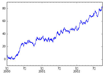
画图
ts = pd.Series(np.random.randn(1000),
index=pd.date_range('1/1/2000', periods=1000))
ts = ts.cumsum()
%matplotlib inline
ts.plot()
<matplotlib.axes._subplots.AxesSubplot at 0x7f7584dafc90>
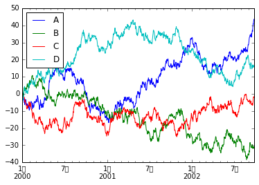
df = pd.DataFrame(np.random.randn(1000, 4), index=ts.index,
columns=['A', 'B', 'C', 'D'])
df = df.cumsum()
plt.figure(); df.plot();
plt.legend(loc='best')
<matplotlib.legend.Legend at 0x7f7574834e50>


<matplotlib.figure.Figure at 0x7f7584daf310>
读取和保存数据
CSV:
df.to_csv(‘foo.csv’)
pd.read_csv(‘foo.csv’)
HDF5:
df.to_hdf(‘foo.h5’,’df’)
pd.read_hdf(‘foo.h5’,’df’)
Excel:
df.to_excel(‘foo.xlsx’, sheet_name=’Sheet1’)
pd.read_excel(‘foo.xlsx’, ‘Sheet1’, index_col=None, na_values=[‘NA’])
附录
本文是对pandas 0.18.1 documentation进行学习的一次学习记录。
原文见10 Minutes to pandas。虽然号称10分钟入门,但也只限于水过地皮湿的理解程度或作为手头的应急查阅文件。我在jupyter-notebook中一步一步按照代码敲下来,边学边理解大概需要四个小时。


 这篇博客介绍了pandas的基本操作,包括创建DataFrame、查看数据、选择数据、处理缺失值、运算、数据融合、分组、时间序列分析以及读写数据等。通过实例展示了如何使用pandas进行数据处理和分析,适合初学者入门。


 1272
1272

 被折叠的 条评论
为什么被折叠?
被折叠的 条评论
为什么被折叠?
 到【灌水乐园】发言


