从说话人识别demo开始学习kaldi--（7）EER的计算

参考这里：
https://blog.csdn.net/zjm750617105/article/details/52558779

我的1.txt长这个样子：（可参考local/prepare_for_eer.py，但我是用excel弄出来的，哈哈），一共14232行。这是整合真实值与打分得到的文件。。

5.1663/target
-32.37284/nontarget
-38.94157/nontarget
-58.89211/nontarget
-69.29233/nontarget

下面先用kaldi的方法计算一下eer：

def read_file(filepath):
    with open(filepath, 'r') as f:
        lines = f.readlines()
    return lines

score_path = r"E:\share_with_ubuntu\aishell-v1\1.txt"
score_lines = read_file(score_path)
target_scores = []
nontarget_scores = []
for line in score_lines:
    splits = line.strip().split('/')
    if splits[1] == 'target':
        target_scores.append(eval(splits[0]))
    else:
        nontarget_scores.append(eval(splits[0]))
print(len(target_scores),len(nontarget_scores))

结果：

7116 135204

kaldi中对于阈值的选择是对target_scores的每一个分数进行迭代，也就是把每一个target_scores中的分数都当做阈值来算一遍。

但是也有文章说，直接在target_scores的最小值和最大值之间取10000个点，把每一个点都当做阈值进行迭代。

设一万个点的可以参考下面：
https://blog.csdn.net/zjm750617105/article/details/60503253
（这里面是对all_scores而不是target_scores分10000个点，到底应该对什么分一万个点呢？我实验了两种，一是对all_scores分一万个点，二是对target_scores分一万个点，但结果几乎是一样的。是真的没有区别还是只是对我的数据没有区别？）

通过对nist，det curve工具（https://www.nist.gov/itl/iad/mig/tools）
的分析得知，nist给的工具中使用的是对all_scores划分阈值，有多少点就有多少待选的阈值。

#从小到大排序
target_scores = sorted(target_scores)
nontarget_scores = sorted(nontarget_scores)

# 下面是kaldi中compute-eer的方法
target_size = len(target_scores)
target_position = 0
for target_position in range(target_size):
    nontarget_size = len(nontarget_scores)
    nontarget_n = nontarget_size * target_position * 1.0 / target_size
    nontarget_position = int(nontarget_size - 1 - nontarget_n)
    if nontarget_position < 0:
        nontarget_position = 0
    if nontarget_scores[nontarget_position] < target_scores[target_position]:
        print ("nontarget_scores[nontarget_position] is",  nontarget_position, nontarget_scores[nontarget_position])
        print ("target_scores[target_position] is",  target_position, target_scores[target_position])
        break

threshold = target_scores[target_position]
print ("threshold is --> ",  threshold)
eer = target_position * 1.0 / target_size
print ("eer is --> ",  eer)

结果：

nontarget_scores[nontarget_position] is 133246 -13.30128
target_scores[target_position] is 103 -13.16873
threshold is -->  -13.16873
eer is -->  0.01447442383361439

但是我不太理解上面的方法，根据下面kaldi中的注释，我们来自己写一下python代码。
ComputeEer computes the Equal Error Rate (EER) for the given scores
and returns it as a proportion beween 0 and 1.
If we set the threshold at x, then the target error-rate is the
proportion of target_scores below x; and the non-target error-rate
is the proportion of non-target scores above x. We seek a
threshold x for which these error rates are the same; this
error rate is the EER.
We compute this by iterating over the positions in target_scores: 0, 1, 2,
and so on, and for each position consider whether the cutoff could be here.
For each of these position we compute the corresponding position in
nontarget_scores where the cutoff would be if the EER were the same.
For instance, if the vectors had the same length, this would be position
length() - 1, length() - 2, and so on. As soon as the value at that
position in nontarget_scores at that position is less than the value from target_scores, we have our EER.

这里再来明确一下FR和FA的定义：
FR = 所有真正例中被判为负例的数目 / 所有真正例的数目。即miss，未命中。
FA = 所有真负例中被判为正例的数目 / 所有真负例的数目。即fa，false-alarm，假警报。

阈值一旦设定，所有小于阈值的都被预测为负例，所有大于阈值的都被预测为正例
这里（真实值中）所有正例的数目就是7116，所有负例的数目就是135204
由于FR和FA不可能完全相等，下面计算他们差的绝对值的最小值。
（或者用插值的方法来求FR和FA完全相等的地方。插值是离散函数逼近的重要方法，利用它可通过函数在有限个点处的取值状况，估算出函数在其他点处的近似值。 from scipy.interpolate import interp1d）

def count_xiaoyu_x(list1,x): # 要求list1是从小到大排列的
    num =0
    for i in range(len(list1)):
        if (list1[i]<x):
            num+=1
        else:
            break
    return num

def count_dayu_x(list1,x): # 要求list1是从小到大排列的
    num =0
    length = len(list1)
    for i in range(length):
        if (list1[length-i-1]>x):
            num+=1
        else:
            break
    return num

fr_list = []
fa_list = []
cha_list = []
for position in range(7116):
    FR = count_xiaoyu_x(target_scores,target_scores[position])/7116
    FA = count_dayu_x(nontarget_scores,target_scores[position])/135204
    cha = abs(FR-FA)
    fr_list.append(FR)
    fa_list.append(FA)
    cha_list.append(cha)

a = min(cha_list)
b = cha_list.index(a)
print(target_scores[b],fr_list[b],fa_list[b],'%.10f'%a)

结果：

-13.22655 0.01433389544688027 0.014363480370403242 0.0000295849

这里发现与kaldi的结果不太一样，刚好是kaldi结果的上一个点
这个cha的变化趋势是怎样的呢，是不是只有一个最低点呢，画个图看看

import numpy as np
import matplotlib.pyplot as plt

fig, ax = plt.subplots()
plt.xlabel('threshhold')
plt.ylabel('cha')  

ax.set_xlim([min(target_scores), max(target_scores)])
ax.set_ylim([min(cha_list), max(cha_list)])

plt.plot(target_scores,cha_list,'.',label=" cha with threshold")

plt.legend(loc='upper right')
plt.show()

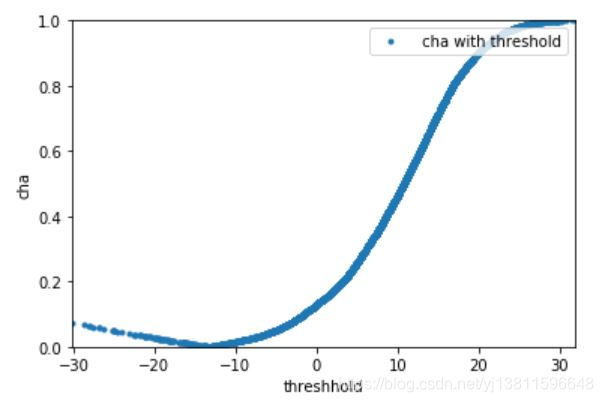
确实只有一个最低点，下面这个才是kaldi的结果

print(target_scores[b+1],fr_list[b+1],fa_list[b+1],'%.10f'%cha_list[b+1])

结果：

-13.16873 0.01447442383361439 0.014274725599834325 0.0001996982

比较两个cha，0.0000295849和0.0001996982，我的结果确实更小一些呢。

现在来画fa和fr随阈值变化的曲线，最好能从曲线上就找到FR和FA离的最近的两个点

#!coding=utf-8
import numpy as np
import matplotlib.pyplot as plt

fig, ax = plt.subplots()
plt.title(" curve")
plt.xlabel('threshhold')
plt.ylabel('y')  

ax.set_xlim([min(target_scores), max(target_scores)])
ax.set_ylim([0, 1])

plt.plot(target_scores,fr_list,'.',label=" FR with threshold")
plt.plot(target_scores,fa_list,'.',label=" FA with threshold")

plt.legend(loc='upper right')
plt.show()

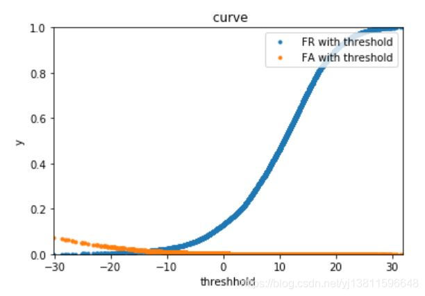
上面的图太不清楚了，怎么能从图上就找到这个交点呢，更改刻度再画一次

a=[]
b=[]
c=[]

for i in range(len(target_scores)):
    if((-20<target_scores[i]) & (target_scores[i]<-10)):
        a.append(target_scores[i])
        b.append(fr_list[i])
        c.append(fa_list[i])
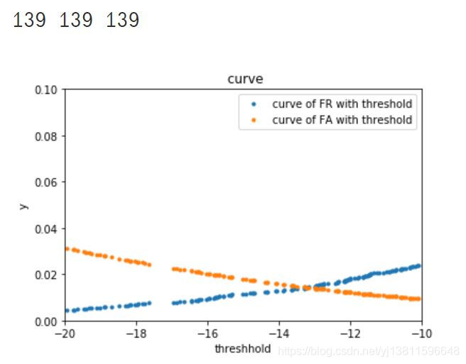
print(len(a),len(b),len(c))

import numpy as np
import matplotlib.pyplot as plt

fig, ax = plt.subplots()
plt.title(" curve")
plt.xlabel('threshhold')
plt.ylabel('y')  

ax.set_xlim([-20, -10])
ax.set_ylim([0, 0.1])

plt.plot(a,b,'.',label="curve of FR with threshold")
plt.plot(a,c,'.',label="curve of FA with threshold")

plt.legend(loc='upper right')
plt.show()

结果：

# 再画一次
a=[]
b=[]
c=[]

for i in range(len(target_scores)):
    if((-14<target_scores[i]) & (target_scores[i]<-12)):
        a.append(target_scores[i])
        b.append(fr_list[i])
        c.append(fa_list[i])

print(len(a),len(b),len(c))

plt.title(" curve")
plt.xlabel('threshhold')
plt.ylabel('y')  

ax.set_xlim([-14, -12])
ax.set_ylim([0, 0.04])

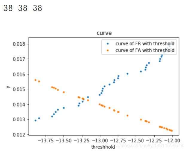
plt.plot(a,b,'.',label="curve of FR with threshold")
plt.plot(a,c,'.',label="curve of FA with threshold")

plt.legend(loc='upper right')
plt.show()
# 这时有38个点，还是不太清楚

# 再画一次
a=[]
b=[]
c=[]

for i in range(len(target_scores)):
    if((-13.5<target_scores[i]) & (target_scores[i]<-13)):
        a.append(target_scores[i])
        b.append(fr_list[i])
        c.append(fa_list[i])

print(len(a),len(b),len(c))

plt.title(" curve")
plt.xlabel('threshhold')
plt.ylabel('y')  

ax.set_xlim([-13.5, -13])
ax.set_ylim([0.013, 0.016])

plt.plot(a,b,'.',label="curve of FR with threshold")
plt.plot(a,c,'.',label="curve of FA with threshold")

plt.legend(loc='upper right')
plt.show()

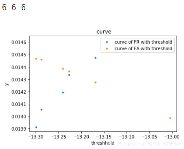
这时只有6个点，可以很清楚的看到第4个点，黄色和蓝色是离的最近的

print(a[3],b[3],c[3])
# 打印出来的阈值，fr，fa和我们上面的计算结果是一样的

结果：

-13.22655 0.01433389544688027 0.014363480370403242

果然和我上面的结果是一样的。

下面画DET曲线，横轴是fa，纵轴是fr

# 先来看下坐标范围
print(min(fa_list),max(fa_list))
print(min(fr_list),max(fr_list))
print(len(fa_list),len(fr_list))

0.0 0.07365906334132126
0.0 0.9998594716132658
7116 7116

# 下面画DET曲线，横轴是fa，纵轴是fr
plt.xlabel('fa')
plt.ylabel('fr')  

ax.set_xlim([0, max(fa_list)])
ax.set_ylim([0, max(fr_list)])

plt.plot(fa_list,fr_list,'.',label="curve of DET")

plt.legend(loc='upper right')
plt.show()

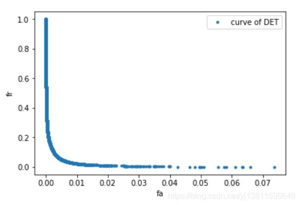
怎么把我们找到的eer的值标记上去呢
参考：python显示图上每个点的坐标：https://zhidao.baidu.com/question/1388281986500209380.html
参考：Python:给图形中添加文本注释（text函数）：https://blog.csdn.net/weixin_38725737/article/details/82664096

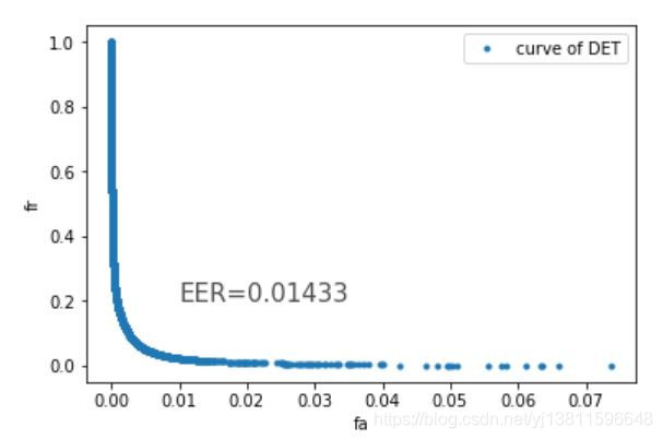
# 怎么把我们找到的eer的值标记上去呢
# 参考：python显示图上每个点的坐标：https://zhidao.baidu.com/question/1388281986500209380.html
# 参考：Python:给图形中添加文本注释（text函数）：https://blog.csdn.net/weixin_38725737/article/details/82664096

plt.xlabel('fa')
plt.ylabel('fr')  

ax.set_xlim([0, max(fa_list)])
ax.set_ylim([0, max(fr_list)])

plt.plot(fa_list,fr_list,'.',label="curve of DET")
plt.text(0.01, 0.2, "EER=0.01433", size = 15, alpha = 0.7)

plt.legend(loc='upper right')
plt.show()

但是下面这个曲线与y=x的交点处横坐标，明显小于0.01啊，为什么呢，难道是因为7116个点太密了？

那再放大一点看细节

m=[]
n=[]

for i in range(len(fa_list)):
    if((0<fa_list[i]) & (fa_list[i]<0.002)):
        m.append(fa_list[i])
        n.append(fr_list[i])
        
print(len(m),len(n))

plt.title(" curve")
plt.xlabel('fa')
plt.ylabel('fr')  

ax.set_xlim([0,0.002])
ax.set_ylim([0,0.2])

plt.plot(m,n,'.',label="curve of DET")

plt.legend(loc='upper right')
plt.show()

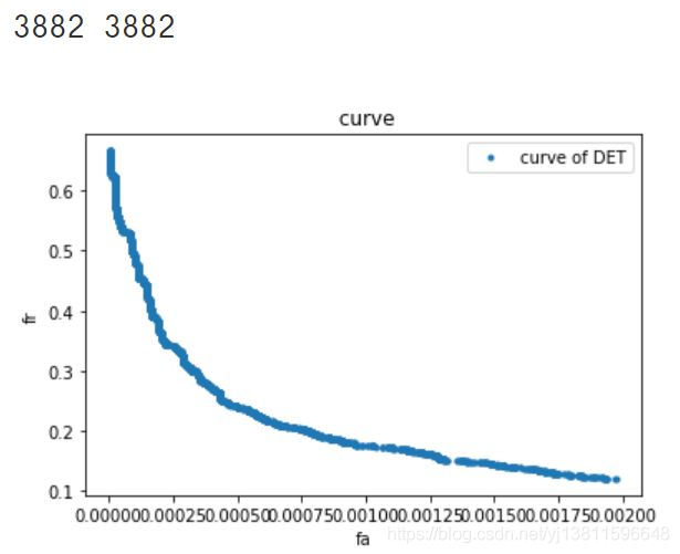
还是这样啊，为什么呢？难道是我画DET曲线的方法不对？

2019.12.16增加：
原来是我的刻度问题，现在把x轴和y轴的刻度弄一样，再画一下：

import numpy as np
import matplotlib.pyplot as plt
# 下面画DET曲线，横轴是fa，纵轴是fr
plt.xlabel('fa')
plt.ylabel('fr')  

#ax.set_xlim([0, 0.08])
#ax.set_ylim([0, 0.08])
plt.xlim(0,0.08)
plt.ylim(0,0.08)

plt.plot(fa_list,fr_list,'.',label="curve of DET")

plt.legend(loc='upper right')
plt.show()

结果：

这下，曲线与对角线y=x的交点有点像在x=0.0143的位置了吧，又有一个新问题了，为啥它画出来不是正方形的图片，怎么是个长方形的？

本页有一个问题没解决：
1.如何理解kaldi中的方法？

------------------2020-11-26–附上另一种计算方法-------------------

def compute_det_curve(target_scores, nontarget_scores):

    n_scores = target_scores.size + nontarget_scores.size
    all_scores = np.concatenate((target_scores, nontarget_scores))
    labels = np.concatenate((np.ones(target_scores.size), np.zeros(nontarget_scores.size)))

    # Sort labels based on scores
    indices = np.argsort(all_scores, kind='mergesort')  # 返回排序后数组的原索引值
    labels = labels[indices]  # 对all_scores从小到大排序后，里面的score就乱了，label也需要重新调整

    # Compute false rejection and false acceptance rates
    tar_trial_sums = np.cumsum(labels)
    # 求累计和
	# 所有真正例的数目
	# 所有真负例的数目
	
	# FR = 所有真正例中被判为负例的数目 / 所有真正例的数目。即miss，未命中。
	# FA = 所有真负例中被判为正例的数目 / 所有真负例的数目。即fa，false-alarm，假警报。
	
	# 有多少分数，就有多少个阈值，有了阈值之后，小于它的，都被判为负例，所有大于它的，都被判为正例
	# 也就是，阈值位置之前，有多少个1，就是所有真正例中被判为负例的数目
	# 阈值位置之后，有多少个0，就是所有真负例中被判为正例的数目
	# 假如阈值选定的是第三个score，位置参数是2，那么在labels[2]之前有几个1呢，通过tar_trial_sums[2]-1=2,我们知道，有2个1
	# 在labels[2]之后有几个0呢，nontarget_trial_sums[2]=155,告诉我们有155个0
    nontarget_trial_sums = nontarget_scores.size - (np.arange(1, n_scores + 1) - tar_trial_sums)

    frr = np.concatenate((np.atleast_1d(0), tar_trial_sums / target_scores.size))  # false rejection rates
    far = np.concatenate((np.atleast_1d(1), nontarget_trial_sums / nontarget_scores.size))  # false acceptance rates
    thresholds = np.concatenate((np.atleast_1d(all_scores[indices[0]] - 0.001), all_scores[indices]))  # Thresholds are the sorted scores

    return frr, far, thresholds


def compute_eer(target_scores, nontarget_scores):
    """ Returns equal error rate (EER) and the corresponding threshold. """
    frr, far, thresholds = compute_det_curve(target_scores, nontarget_scores)
    abs_diffs = np.abs(frr - far) # 求差的最小值，即找离的最近的两个点
    min_index = np.argmin(abs_diffs) # 求最小值所在的位置
    eer = np.mean((frr[min_index], far[min_index]))  # 求均值
    return eer, thresholds[min_index]

---------------------2020.12.1-------------------------------

from scipy.optimize import brentq
from scipy.interpolate import interp1d
from sklearn.metrics import roc_curve, confusion_matrix

# EER reference: https://yangcha.github.io/EER-ROC/

def compute_eer(y_true, y_pred):
    fpr, tpr, _ = roc_curve(y_true, y_pred, pos_label=1)
    eer = brentq(lambda x : 1. - x - interp1d(fpr, tpr)(x), 0., 1)
    
    return 100. * eer

def compute_confuse(y_true, y_pred):
    return confusion_matrix(y_true, y_pred)