


#coding:utf-8
import numpy as np
from sklearn.covariance import EllipticEnvelope
from sklearn.svm import OneClassSVM
import matplotlib.pyplot as plt
import matplotlib.font_manager
from sklearn.datasets import load_boston
'''
机器学习 鲁棒的基于高斯概率密度的异常点检测(novelty detection) ellipticalenvelope算法

算法理解:
这个算法的思想很好理解, 就是求出训练集在空间中的重心, 和方差, 然后根据高斯概率密度估算每个点被分配到重心的概率.

数据说明:
[
0CRIM,城镇人均犯罪率,
1ZN,占地面积超过25,000平方呎的住宅用地比例,
2INDUS,每个城镇非零售商业地的比例,
3,查尔斯河虚拟变量(= 1有河;否则为0),
4,一氧化氮浓度(百万分之一),
5,每间住宅的平均客房数,
6,1940年之前建成的自用单位比例,
7,加权距离到五个波士顿就业中心,
8,径向公路的可达性指数,
9,每10,000美元的税赋全值财产税率,
10,学生与教师的比率,
11,1000*(Bk-0.63)^2 其中Bk是城镇中黑人的比例,
12,%降低人口状态,
13,自住房价值在1000美元的中位数,[数据不包含该项]
]
['CRIM', 'ZN', 'INDUS', 'CHAS', 'NOX', 'RM', 'AGE', 'DIS', 'RAD','TAX', 'PTRATIO', 'B', 'LSTAT']
[0.00632, 18.0, 2.31, 0.0, 0.538, 6.575, 65.2, 4.09, 1.0, 296.0, 15.3, 396.9, 4.98]
'''
# Get data
#X1[径向公路的可达性指数,学生与教师的比率,]
X1 = load_boston()['data'][:, [8, 10]]  # two clusters
#X2[每间住宅的平均客房数,降低人口状态,]
X2 = load_boston()['data'][:, [5, 12]]  # "banana"-shaped

# Define "classifiers" to be used
classifiers = {
    #EllipticEnvelope:一种用于在高斯分布式数据集中检测异常值的对象。contamination:数据集的污染量,即数据集中异常值的比例。
    u"经验协方差": EllipticEnvelope(support_fraction=1,contamination=0.261),
    #基于协方差的稳健估计,假设数据是高斯分布的,那么在这样的案例中执行效果将优于One-Class SVM;
    u"鲁棒协方差(最小协方差决定因素)":EllipticEnvelope(contamination=0.261),
    #SVM 利用One-Class SVM,它有能力捕获数据集的形状,因此对于强非高斯数据有更加优秀的效果,例如两个截然分开的数据集;
    "OCSVM": OneClassSVM(nu=0.261, gamma=0.05)}
colors = ['m', 'g', 'b']
legend1 = {}
legend2 = {}

# Learn a frontier for outlier detection with several classifiers
xx1, yy1 = np.meshgrid(np.linspace(-8, 28, 500), np.linspace(3, 40, 500))
xx2, yy2 = np.meshgrid(np.linspace(3, 10, 500), np.linspace(-5, 45, 500))
for i, (clf_name, clf) in enumerate(classifiers.items()):
    plt.figure(1)
    clf.fit(X1)
    #decision_function 计算给定观察的决策函数
    #我们知道数据集中一部分的异常值。由此我们通过对decision_function设置阈值来分离出相应的部分,而不是使用'预测'方法。
    Z1 = clf.decision_function(np.c_[xx1.ravel(), yy1.ravel()])
    #reshape 将Z1矩阵转换成 xx1的行列形式
    Z1 = Z1.reshape(xx1.shape)
    #画函数图像的 contour:表示绘制轮廓 使数组的等值线图。水平值自动选择。
    legend1[clf_name] = plt.contour(xx1, yy1, Z1, levels=[0], linewidths=2, colors=colors[i])
    plt.figure(2)
    clf.fit(X2)
    Z2 = clf.decision_function(np.c_[xx2.ravel(), yy2.ravel()])
    Z2 = Z2.reshape(xx2.shape)
    legend2[clf_name] = plt.contour(xx2, yy2, Z2, levels=[0], linewidths=2, colors=colors[i])

legend1_values_list = list(legend1.values())
legend1_keys_list = list(legend1.keys())

# Plot the results (= shape of the data points cloud)
plt.figure(1)  # two clusters
plt.title(u"实际数据集(波士顿房屋)的异常值检测")
#画点图
plt.scatter(X1[:, 0], X1[:, 1], color='red')

#设置注释文本框 fc设置透明度
bbox_args = dict(boxstyle="round", fc="0.8")
#arrow_args 表示使用箭头线
arrow_args = dict(arrowstyle="->")
#控制注解 xy=(24,19)表示箭头的终点位置 xytext=(13, 10)注解文本框的位置
plt.annotate(u"一些混淆的点", xy=(24, 19),xycoords="data", textcoords="data",xytext=(13, 10), bbox=bbox_args, arrowprops=arrow_args)
plt.xlim((xx1.min(), xx1.max()))
plt.ylim((yy1.min(), yy1.max()))

#loc 控制说明的摆放位置
plt.legend((legend1_values_list[0].collections[0],
            legend1_values_list[1].collections[0],
            legend1_values_list[2].collections[0]),
           (legend1_keys_list[0], legend1_keys_list[1], legend1_keys_list[2]),
           loc="upper center",
           prop=matplotlib.font_manager.FontProperties(size=12))
plt.ylabel(u"径向公路的可达性指数")
plt.xlabel(u"学生与教师的比率")

legend2_values_list = list(legend2.values())
legend2_keys_list = list(legend2.keys())

plt.figure(2)  # "banana" shape
plt.title("Outlier detection on a real data set (boston housing)")
plt.scatter(X2[:, 0], X2[:, 1], color='black')
plt.xlim((xx2.min(), xx2.max()))
plt.ylim((yy2.min(), yy2.max()))
plt.legend((legend2_values_list[0].collections[0],
            legend2_values_list[1].collections[0],
            legend2_values_list[2].collections[0]),
           (legend2_keys_list[0], legend2_keys_list[1], legend2_keys_list[2]),
           loc="upper center",
           prop=matplotlib.font_manager.FontProperties(size=12))
plt.ylabel("% lower status of the population")
plt.xlabel("average number of rooms per dwelling")

plt.show()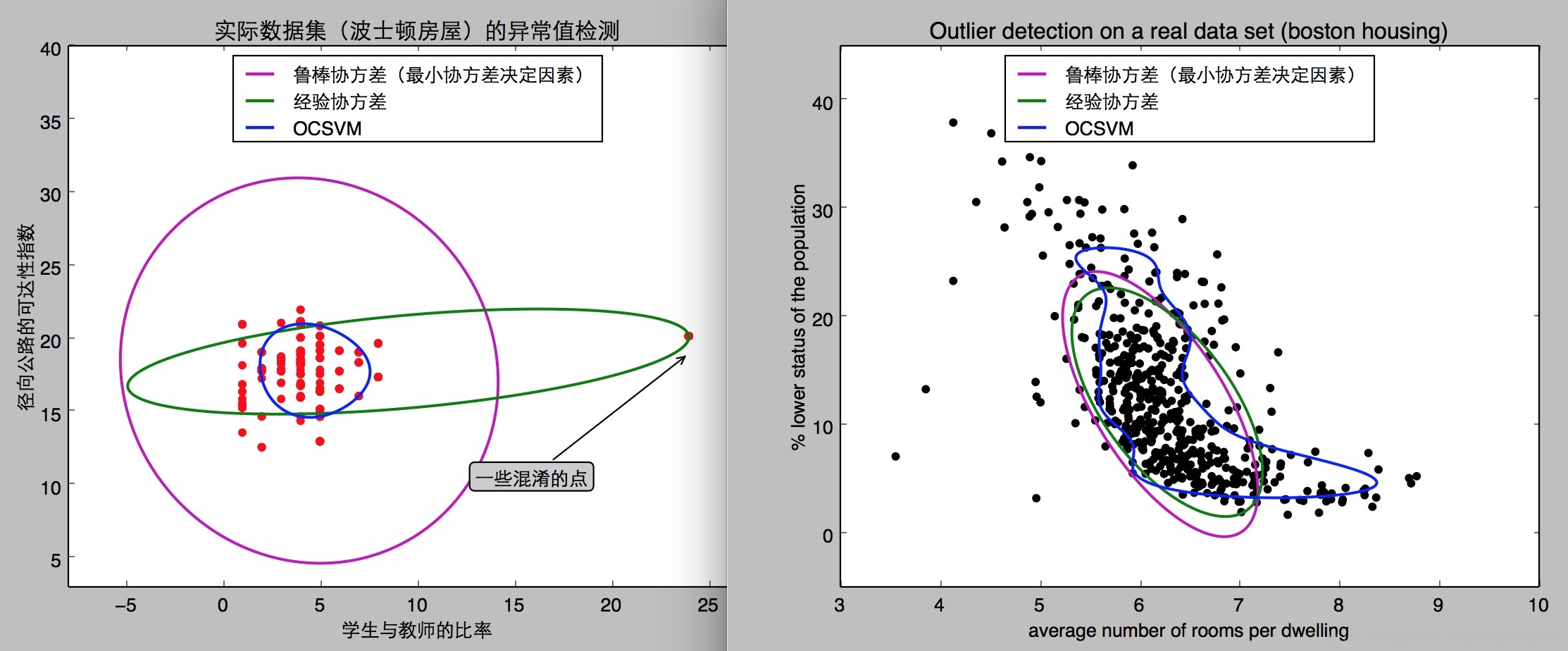


 281
281


 被折叠的 条评论
为什么被折叠?
被折叠的 条评论
为什么被折叠?
 到【灌水乐园】发言


