


/* 已知X,Y,利用最小二乘法估计回归方程Y=XB+E */
*ods trace output;
proc iml;
start reg;
   n = nrow(x);  /* 观测值数目 */
   k = ncol(x);    /* 变量数目 */
   xpx = x`*x;         /* 内积 */
   xpy = x`*y;
   xpxi = inv(xpx); /* 内积矩阵的逆矩阵 */
   b = xpxi*xpy;    /* 参数b的估计 */
   yhat = x*b;      /* y的预测值 */
   resid = y-yhat;  /* 真实值预测值残差 */
   sse = resid`*resid; /* 残差平方和*/
   dfe = n-k; /* 残差的自由度 */
   mse = sse/dfe; /* 均方误差 */
   rmse = sqrt(mse); /*均方标准差 */
   covb = xpxi#mse; /* 估计值b的协方差 */
   stdb = sqrt(vecdiag(covb)); /* 标准误差 */
   t = b/stdb; /* 估计值的t检验,零假设b=0 */
   probt = 1-probf(t#t,1,dfe); /* t检验有显著性的p值 */
   print name b stdb t probt;
   s = diag(1/stdb);
   corrb = s*covb*s; /* 估计值的相关系数矩阵 */
   print ,"Covariance of Estimates", covb[r=name c=name] ,
          "Correlation of Estimates",corrb[r=name c=name] ;
   if nrow(tval)=0 then return; /* 设定t值 */
      projx = x*xpxi*x`; /* hat matrix */
      vresid = (i(n)-projx)*mse; /* covariance of residuals */
      vpred = projx#mse; /* covariance of predicted values */
      h = vecdiag(projx); /* hat leverage values */
      lowerm = yhat-tval#sqrt(h*mse); /* low. conf lim for mean */
      upperm = yhat+tval#sqrt(h*mse); /* upper lim. for mean */
      lower = yhat-tval#sqrt(h*mse+mse); /* lower lim. for indiv*/

      upper = yhat+tval#sqrt(h*mse+mse);/* upper lim. for indiv */
      print ,,"Predicted Values, Residuals, and Limits" ,,
              y yhat resid h lowerm upperm lower upper;
finish reg;

/* Routine to test a linear combination of the estimates */
/* given L, this routine tests hypothesis that LB = 0. */
start test;
   dfn=nrow(L);
   Lb=L*b;
   vLb=L*xpxi*L`;
   q=Lb`*inv(vLb)*Lb /dfn;
   f=q/mse;
   prob=1-probf(f,dfn,dfe);
print ,f dfn dfe prob;
finish test;
/* Run it on population of U.S. for decades beginning 1790 */
x= { 1 1 1,
     1 2 4,
     1 3 9,
     1 4 16,
     1 5 25,
     1 6 36,
     1 7 49,
     1 8 64 };
y= {3.929,5.308,7.239,9.638,12.866,17.069,23.191,31.443};
name={"Intercept", "Decade", "Decade**2" };
tval=2.57; /* for 5 df at 0.025 level to get 95% conf. int. */
reset fw=7;
run reg;
do;
print ,"TEST Coef for Linear";
L={0 1 0 };
run test;
print ,"TEST Coef for Linear,Quad";
L={0 1 0,0 0 1};
run test;
print ,"TEST Linear+Quad = 0";
L={0 1 1 };
run test;
end;
线性代数知识梳理
1.Y=XB+E,参数B结果:
PROC IML;
x={1 2,2 3,4 3};
y={-1,-2,-2};
b=INV(x‘*x)*x‘*y;
PRINT b;
QUIT;
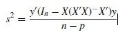
2.方差的最小二乘估计:
PROC IML;
x={1 2,2 3,4 3};
y={-1,-2,-2};
n=NROW(x); /*样本容量n*/
p=ROUND(TRACE(GINV(x)*x)); /*矩阵稚次*/
in=I(n);
s2=(1/(n-p))*y‘*(in-x*GINV(x‘*x)*x‘)*y;
s=SQRT(s2);
PRINT s2 s;
QUIT;
3.矩阵的分解:a.奇异阵分解:![]() ,CALL SVD( )
,CALL SVD( )
Proc IML;
a = {1 2 3 4,
5 6 7 8,
9 0 1 2};
RESET FUZZ;
CALL SVD(u,q,v,a);
upu = u‘*u;
vpv = v‘*v;
vvp = v*v‘;
uup = u*u‘;
a2 = u*DIAG(q)*v‘;
ginva=GINV(a);
m = NROW(a); n = NCOL(a);
DO i=1 TO n;
IF q[i] <= 1E-12 * q[1] then q[i] = 0;
ELSE q[i] = 1 / q[i];
END;
ga = v*DIAG(q)*u‘;
PRINT a a2„ u q v„ upu uup„ vpv vvp„ ginva ga;
QUIT;
b.)施密特正交化,CALL GSORTH()
PROC IML;
a={1 2 3,2 3 5,3 7 11};
CALL GSORTH(p,t,lindep,a);
p_inv=INV(p);
b=p*t;
PRINT a b,p p_inv,t lindep;
QUIT;
4.线性方程求解
• HOMOGEN Function: 解其次线性方程
• SOLVE Function: 解普通线性方程
• TRISOLV Function: 三角形矩阵解方程
a).Solving AX=0 for X:
PROC IML;
RESET FUZZ;
a={10 5 15, 12 6 18, 14 7 21, 16 8 24};
x=HOMOGEN(a);
zero1=a*x[,1];
zero2=a*x[,2];
PRINT a x zero1 zero2;
QUIT;
b).Solving AX=B for X: 区别:x=INV(a)*b;
PROC IML;
a={1 2 3,6 5 4,0 7 8};
b={1, 2, 3};
x=SOLVE(a,b);
ax=a*x;
PRINT a x b ax ;
QUIT;
5.特征值与特征向量
• EIGEN CALL计算特征值和特征向量为方阵
• EIGVAL Function计算特征值为一个方阵
• EIGVEC Function计算特征向量为一个方阵
• GENEIG Call 计算特征值和特征向量为一般矩阵
Proc IML;
a={ 1 0 1,
0 4 -1,
1 -1 2};
RESET FUZZ;
eigval=EIGVAL(a);
rank=ROUND(TRACE(GINV(a)*a)); /** 矩阵A的稚 **/
PRINT a , ,eigval, ,rank;
RESET FUZZ;
CALL EIGEN(eigval,eigvec,a);
ax1=a*eigvec[,1];
ax2=a*eigvec[,2];
ax3=a*eigvec[,3];
lx1=eigval[1]*eigvec[,1];
lx2=eigval[2]*eigvec[,2];
lx3=eigval[3]*eigvec[,3];
PRINT a„eigval„eigvec„ax1 lx1„ax2 lx2„ax3 lx3;
QUIT;


 1万+
1万+

 被折叠的 条评论
为什么被折叠?
被折叠的 条评论
为什么被折叠?
 到【灌水乐园】发言


