回归分析作业2

作业内容：

在http://stat.ethz.ch/R-manual/R-devel/library/datasets/html/longley.html中

对数据Longley's Economic Regression Data进行了介绍，仔细阅读后做如下分析：
(1) 检查复共线性；
(2) 使用主成分回归解决复共线性，选择适当个数的主成分；

(3) 使用岭回归解决复共线性，并采用不同方法估计岭参数。

我的答案（仅供参考）

#1、
kappa(cor(longley[,c(-1,-6)]))
#1746.892>1000 存在严重的复共线性
library(DAAG)
lm.reg<-lm(Employed~GNP+Unemployed+Armed.Forces+Population+Year,data=longley)
vif(lm.reg,digits=4)
#      GNP   Unemployed Armed.Forces   Population         Year 
#    1034.000       23.260        3.152      225.700      732.600  膨胀因子大多大于10，存在严重的相关性

#2、
pca<-princomp(longley[,c(-1,-6)],cor=TRUE)
summary(pca,loadings=TRUE)
#Importance of components:
#                          Comp.1    Comp.2     Comp.3      Comp.4
#Standard deviation     1.8839994 1.0888267 0.50115614 0.110913452
#Proportion of Variance 0.7098908 0.2371087 0.05023149 0.002460359
#Cumulative Proportion  0.7098908 0.9469995 0.99723100 0.999691358
#                            Comp.5
#Standard deviation     0.039283711
#Proportion of Variance 0.000308642
#Cumulative Proportion  1.000000000

#             Comp.1 Comp.2 Comp.3 Comp.4 Comp.5
#GNP          -0.528        -0.179 -0.226  0.798
#Unemployed   -0.352 -0.615  0.665  0.235       
#Armed.Forces -0.235  0.779  0.577              
#Population   -0.527        -0.107 -0.635 -0.550
#Employed     -0.514        -0.426  0.698 -0.242
#选择2-3个主成分即可


#3、
library(MASS)
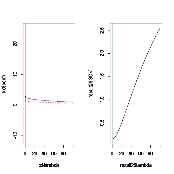
result2<-lm.ridge(Employed~GNP+Unemployed+Armed.Forces+Population+Year,data=longley,data=longley,lambda=seq(0,100,0.01))
result2$lambda[which.min(result2$GCV)]
result2$coef[,which.min(result2$GCV)]
par(mfrow=c(1,2))
plot(result2)
abline(v=result2$lambda[which.min(result2$GCV)],col=2)
plot(result2$lambda,result2$GCV,type="l")
abline(v=result2$lambda[which.min(result2$GCV)],col=3)
select(result2)
#            GNP   Unemployed Armed.Forces   Population         Year 
#    14.5822749    1.4631645    0.4374007   -7.8066243    2.5443023 
#    Employed 
#   -0.1067656 
#使用岭际法得到的参数估计
#modified HKB estimator is 0.006836982 使用HB公式 
#modified L-W estimator is 0.05267247 
#smallest value of GCV  at 0.01 使用岭际法得到的K值