


 本文详细介绍了回归分析的基础,包括一元线性回归和多元线性回归,以及如何在R中建立和诊断模型。讨论了岭回归、LASSO和弹性网等方法解决多重共线性问题。此外,还提到了主成分分析和因子分析在降维中的作用,以及决策树和随机森林等机器学习模型的应用。
一元线性回归模型
创建数组:
> height=c(171,175,159,155,152,158,154,164,168,166,159,164) ;
> y
 [1] 57 64 41 38 35 44 41 51 57 49 47 46
> weight=c(57,64,41,38,35,44,41,51,57,49,47,46)
> summary(height)
   Min. 1st Qu.  Median    Mean 3rd Qu.    Max.
  152.0   157.2   161.5   162.1   166.5   175.0
> height
 [1] 171 175 159 155 152 158 154 164 168 166 159 164
> weight
 [1] 57 64 41 38 35 44 41 51 57 49 47 46
>
相关系数
我们使用相关系数去衡量线性相关性的强弱
## method可以为"spearman","pearson" and "kendall" ,
## 分别对应三种相关系数的计算和检验。
> cor.test(height,weight,method="spearman")

        Spearman's rank correlation rho

data:  height and weight
S = 16.616, p-value = 4.727e-06
alternative hypothesis: true rho is not equal to 0
sample estimates:
      rho
0.9419014

Warning message:
In cor.test.default(height, weight, method = "spearman") :
  无法给连结计算精確p值
> 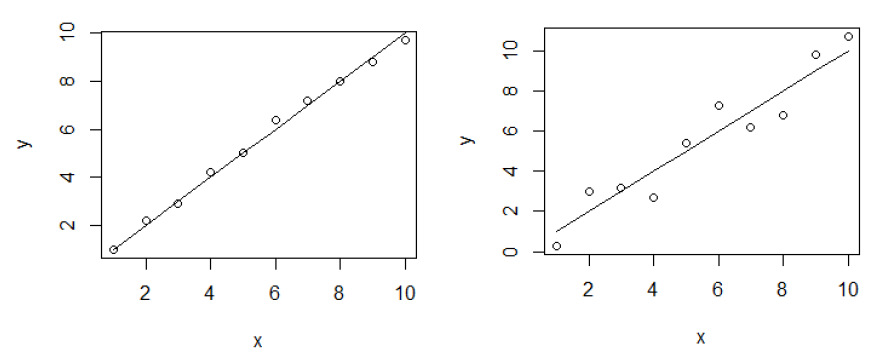
通过计算,左图中的相关系数为0.9930858,右图的相关系数为0.9573288
一元线性回归模型
Y = α + βx + ε (截距项α、斜率β、误差项ε)
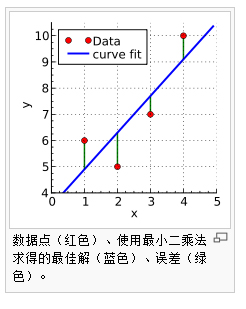
最小二乘法:
1、x=c(1,2,3,4),y=c(6,5,7,10)。构建y关于x的回归方程y=α+βx
2、使用最小二乘法求解参数:
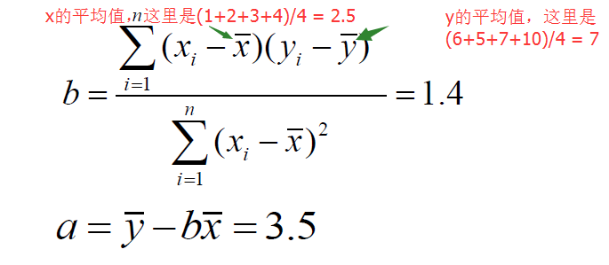
3、得到 y = 3.5 + 1.4x
4、如果有新的点x=2.5,则我们预测相应的y值为3.5+1.4*2.5=7
R建立线性模型(lm()线性模型函数)
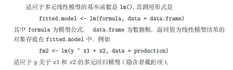
1、y~1+x或y~x均表示y=a+bx有截距形式的线性模型
2、通过原点的线性模型可以表达为:y ~ x -1 或y ~ x + 0 或y ~ 0 + x
3、参见help(formula)
> hw.lm <- lm(weight~height);
> hw.lm

Call:
lm(formula = weight ~ height)

Coefficients:
(Intercept)       height
   -140.364        1.159

> summary(hw.lm)

Call:
lm(formula = weight ~ height)

Residuals:
   Min     1Q Median     3Q    Max
-3.721 -1.699  0.210  1.807  3.074

Coefficients:
             Estimate Std. Error t value Pr(>|t|)
(Intercept) -140.3644    17.5026   -8.02 1.15e-05 ***
height         1.1591     0.1079   10.74 8.21e-07 ***
---
Signif. codes:  0 ‘***’ 0.001 ‘**’ 0.01 ‘*’ 0.05 ‘.’ 0.1 ‘ ’ 1

Residual standard error: 2.546 on 10 degrees of freedom
Multiple R-squared:  0.9203,    Adjusted R-squared:  0.9123
F-statistic: 115.4 on 1 and 10 DF,  p-value: 8.21e-07

//Residuals:参差分析数据
//Coefficients:回归方程的系数,以及推算的系数的标准差,t值,P-值
//F-statistic:F检验值
//Signif:显著性标记,***极度显著,**高度显著,*显著,圆点不太显著,没有记号不显著
>
单因素方差分析ANOVA
> anova(hw.lm)
Analysis of Variance Table

Response: weight
          Df Sum Sq Mean Sq F value   Pr(>F)
height     1 748.17  748.17  115.41 8.21e-07 ***
Residuals 10  64.83    6.48
---
Signif. codes:  0 ‘***’ 0.001 ‘**’ 0.01 ‘*’ 0.05 ‘.’ 0.1 ‘ ’ 1
> swiss.lm

Call:
lm(formula = Fertility ~ ., data = swiss)

Coefficients:
     (Intercept)       Agriculture       Examination         Education          Catholic  Infant.Mortality
         66.9152           -0.1721           -0.2580           -0.8709            0.1041            1.0770

> anova(swiss.lm)
Analysis of Variance Table

Response: Fertility
                 Df  Sum Sq Mean Sq F value    Pr(>F)
Agriculture       1  894.84  894.84 17.4288 0.0001515 ***
Examination       1 2210.38 2210.38 43.0516 6.885e-08 ***
Education         1  891.81  891.81 17.3699 0.0001549 ***
Catholic          1  667.13  667.13 12.9937 0.0008387 ***
Infant.Mortality  1  408.75  408.75  7.9612 0.0073357 **
Residuals        41 2105.04   51.34
---
Signif. codes:  0 ‘***’ 0.001 ‘**’ 0.01 ‘*’ 0.05 ‘.’ 0.1 ‘ ’ 1
>
查看模型系数
> coef(hw.lm)
(Intercept)      height
 -140.36436     1.15906
> coef(swiss.lm)
     (Intercept)      Agriculture      Examination        Education         Catholic Infant.Mortality
      66.9151817       -0.1721140       -0.2580082       -0.8709401        0.1041153        1.0770481
>
提取模型公式
> formula(hw.lm)
weight ~ height
> formula(swiss.lm)
Fertility ~ Agriculture + Examination + Education + Catholic +
    Infant.Mortality
>
计算残差平方和
> deviance(hw.lm)
[1] 64.82657
> deviance(swiss.lm)
[1] 2105.043
>
绘画模型诊断图(很强大,显示残差、拟合值和一些诊断情况)
> plot(hw.lm)计算残差
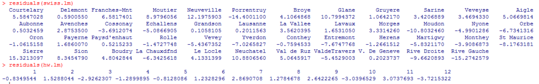
> residuals(hw.lm)
         1          2          3          4          5          6          7
-0.8349544  1.5288044 -2.9262307 -1.2899895 -0.8128086  1.2328296  2.8690708
         8          9         10         11         12
 1.2784678  2.6422265 -3.0396529  3.0737693 -3.7215322
>
作出预测
> data.frame(height=185)
  height
1    185
> h=data.frame(height=185)
> predict(hw.lm,h)
      1
74.0618
关于线性回归的适用范围
1、在身高与体重的例子中,我们注意到得到的回归方程中的截距项为-140.364 ,这表示身高为0的人的体重是负值,这明显是不可能的。所以这个回归模型对于儿童和身高特别矮的人不适用。
2、回归问题擅长内推插值,而不擅长于外推归纳。在使用回归模型做预测时要注意x适用的取值范围
虚拟变量
1、虚拟变量的定义:
- 线性:比如:人类的身高数据、体重数据,虽然在一定范围内但测量值各不相同,变化无穷
- 非线性:对于性别、血型这类样本,并不是线性的,因为可以穷举
- 虚变量:在做线性回归时,需要引入虚变量(哑变量)
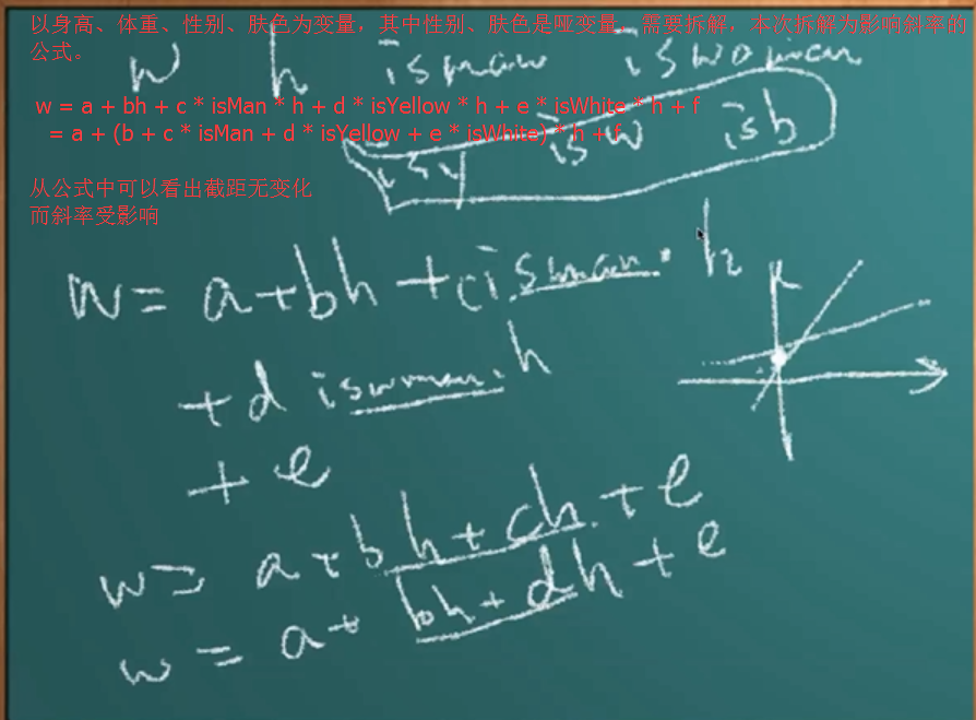
2、虚拟变量的作用:改变曲线截距、斜率
3、虚拟变量的设置:
- 影响方程截距(图片公式有误):
w = a + b*h + c * isMan * + d (离散化非线性变量采用N-1个属性,例如性别有两类,那么2减1,离散化成为一类(isMan),否则会出现强多重共线性)
以上公式一般采用如下变形:
w = a + b * isMan * h + c * isWoman * h

- 影响方程斜率:
- 
- 混合模型:
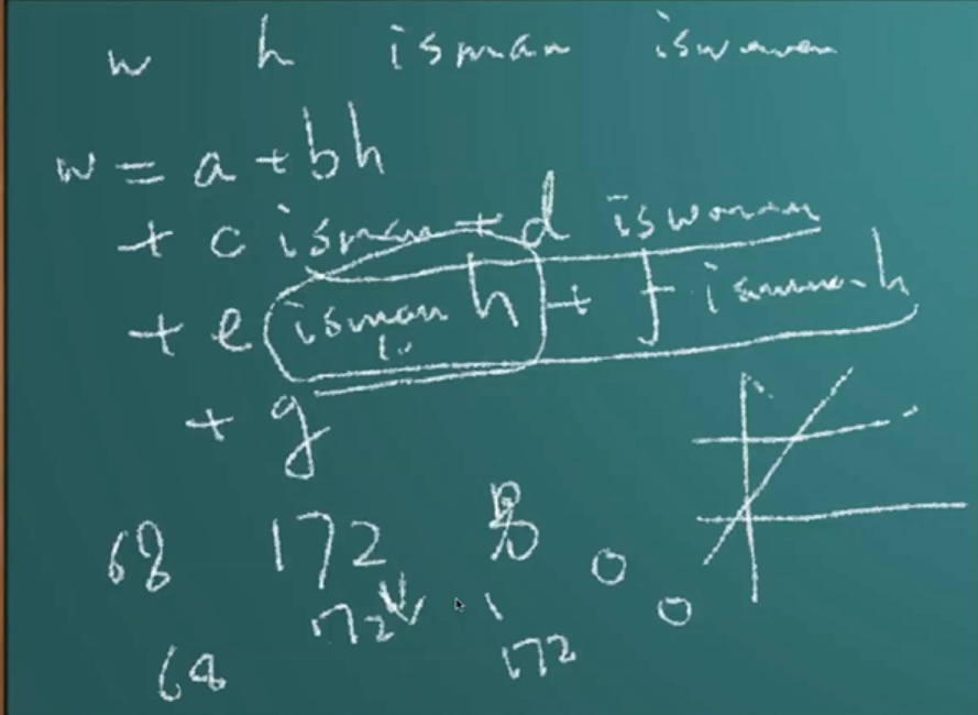
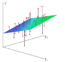
多元线性回归模型
当Y值的影响因素不唯一时,采用多元线性回归模型:

Swiss数据集:Swiss Fertility and Socioeconomic Indicators (1888) Data
> swiss
             Fertility Agriculture Examination Education Catholic Infant.Mortality
Courtelary        80.2        17.0          15        12     9.96             22.2
Delemont          83.1        45.1           6         9    84.84             22.2
Franches-Mnt      92.5        39.7           5         5    93.40             20.2
Moutier           85.8        36.5          12         7    33.77             20.3
Neuveville        76.9        43.5          17        15     5.16             20.6
Porrentruy        76.1        35.3           9         7    90.57             26.6
Broye             83.8        70.2          16         7    92.85             23.6
Glane             92.4        67.8          14         8    97.16             24.9
Gruyere
最低0.47元/天 解锁文章


 1万+
1万+

 被折叠的 条评论
为什么被折叠?
被折叠的 条评论
为什么被折叠?
 到【灌水乐园】发言


