


我比较适合这个

以下英文文档皆出自课程配套笔记
章节一
课3 Supervised Learning
Supervised Learning
In supervised learning, we are given a data set and already know what our correct output
should look like, having the idea that there is a relationship between the input and the output.
Supervised learning problems are categorized into "regression" and "classification" problems.
In a regression problem, we are trying to predict results within a continuous output, meaning
that we are trying to map input variables to some continuous function. In a classification
problem, we are instead trying to predict results in a discrete(离散的) output. In other words, we are
trying to map input variables into discrete categories.
Example 1:
Given data about the size of houses on the real estate market, try to predict their price. Price
as a function of size is a continuous output, so this is a regression problem.
We could turn this example into a classification problem by instead making our output about
whether the house "sells for more or less than the asking price." Here we are classifying the
houses based on price into two discrete categories.
Example 2:
(a) Regression - Given a picture of a person, we have to predict their age on the basis of the
given picture
(b) Classification - Given a patient with a tumor, we have to predict whether the tumor is
malignant or benign.
课4 Unsupervised Learning
Unsupervised learning allows us to approach problems with little or no idea what our resultsshould look like. We can derive(获得) structure from data where we don't necessarily know the
effect of the variables.
We can derive this structure by clustering(聚类) the data based on relationships among the variables
in the data.
With unsupervised learning there is no feedback based on the prediction results.
Example:
Clustering: Take a collection of 1,000,000 different genes, and find a way to automatically
group these genes into groups that are somehow similar or related by different variables,
such as lifespan, location, roles, and so on.
Non-clustering: The "Cocktail Party Algorithm", allows you to find structure in a chaotic
environment. (i.e. identifying individual voices and music from a mesh of sounds at a cocktail
party).
章节二 单变量线性回归
课6 模型描述
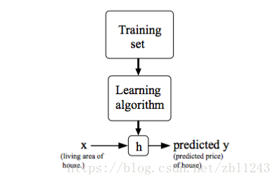
Model RepresentationTo establish notation for future use, we’ll use x ( i ) to denote the “input” variables (living
area in this example), also called input features, and y ( i ) to denote the “output” or target
variable that we are trying to predict (price). A pair ( x ( i ), y ( i )) is called a training example, and
the dataset that we’ll be using to learn—a list of m training examples ( x ( i ), y ( i )); i =1,..., m —is
called a training set. Note that the superscript “(i)” in the notation is simply an index into
the training set, and has nothing to do with exponentiation. We will also use X to denote the
space of input values, and Y to denote the space of output values. In this example, X = Y = ℝ.
To describe the supervised learning problem slightly more formally, our goal is, given a
training set, to learn a function h : X → Y so that h(x) is a “good” predictor for the
corresponding value of y. For historical reasons, this function h is called a hypothesis. Seen
pictorially, the process is therefore like this:
When the target variable that we’re trying to predict is continuous, such as in our housing
example, we call the learning problem a regression problem. When y can take on only a small
number of discrete values (such as if, given the living area, we wanted to predict if a dwelling
is a house or an apartment, say), we call it a classification problem.
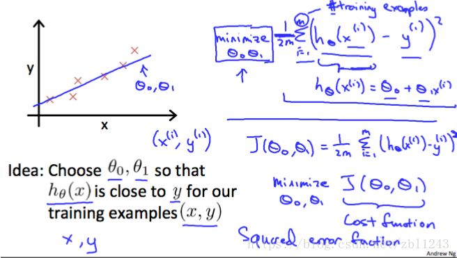
We can measure the accuracy of our hypothesis(假设) function by using a cost function. This takes
an average difference (actually a fancier version of an average) of all the results of the
hypothesis with inputs from x's and the actual output y's.
J ( θ 0, θ 1)=1/(2 m) ∑ i =从1 到m的累加 ( y ^ i − yi )平方=12 m ∑ i =1 m ( hθ ( xi )− yi )2--------这里格式混乱 见下图
To break it apart, it is 12 x ¯ where x ¯ is the mean of the squares of hθ ( xi )− yi , or the difference
between the predicted value and the actual value.
This function is otherwise called the "Squared error function", or "Mean squared error". The
mean is halved (12)as a convenience for the computation of the gradient descent, as the
derivative term of the square function will cancel out the 12 term. The following image
summarizes what the cost function does:
example, we call the learning problem a regression problem. When y can take on only a small
number of discrete values (such as if, given the living area, we wanted to predict if a dwelling
is a house or an apartment, say), we call it a classification problem.
课7 代价函数
Cost FunctionWe can measure the accuracy of our hypothesis(假设) function by using a cost function. This takes
an average difference (actually a fancier version of an average) of all the results of the
hypothesis with inputs from x's and the actual output y's.
J ( θ 0, θ 1)=1/(2 m) ∑ i =从1 到m的累加 ( y ^ i − yi )平方=12 m ∑ i =1 m ( hθ ( xi )− yi )2--------这里格式混乱 见下图
To break it apart, it is 12 x ¯ where x ¯ is the mean of the squares of hθ ( xi )− yi , or the difference
between the predicted value and the actual value.
This function is otherwise called the "Squared error function", or "Mean squared error". The
mean is halved (12)as a convenience for the computation of the gradient descent, as the
derivative term of the square function will cancel out the 12 term. The following image
summarizes what the cost function does:
课8 代价函数一
Cost Function - Intuition IIf we try to think of it in visual terms, our training data set is scattered on the x-y plane. We
are trying to make a straight line (defined by hθ ( x )) which passes through these scattered data
points.
Our objective is to get the best possible line. The best possible line will be such so that the
average squared vertical distances of the scattered points from the line will be the least. Ideally,
the line should pass through all the points of our training data set. In such a case, the value
of J ( θ 0, θ 1) will be 0. The following example shows the ideal situation where we have a cost
function of 0.
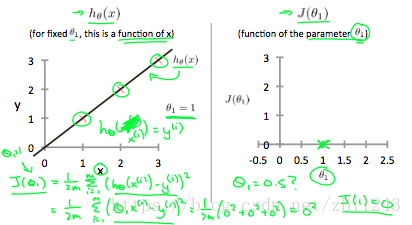
When θ 1=1, we get a slope of 1 which goes through every single data point in our model.
Conversely, when θ 1=0.5, we see the vertical distance from our fit to the data points increase.
Conversely, when θ 1=0.5, we see the vertical distance from our fit to the data points increase.
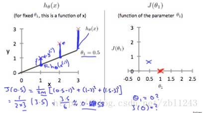
This increases our cost function to 0.58. Plotting several other points yields to the following
graph:
graph:
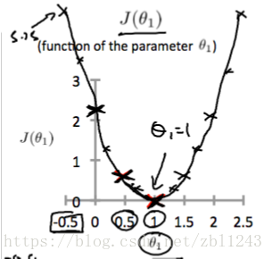
Thus as a goal, we should try to minimize the cost function. In this case, θ 1=1 is our global
minimum.
minimum.


 1422
1422

 被折叠的 条评论
为什么被折叠?
被折叠的 条评论
为什么被折叠?
 到【灌水乐园】发言


