Kaggle经典项目——房价预测

写在前面：
这篇文章旨在梳理kaggle回归问题的一个基本流程。博主只是一个数据分析刚入门的新手，有些错漏之处还请批评指正。很遗憾这个项目最后提交的Private Score只达到了排行榜的TOP13%，我目前也还没有更好的方法去进一步提高分数，不过整个项目做完之后对kaggle回归预测项目的解题思路有了一套比较完整清楚的认识，总结出来和大家分享，欢迎共同探讨。
完整的代码放在github：kaggle房价预测完整代码

1.项目背景

问题陈述

房价预测是kaggle的一个经典Data Science项目，作为数据分析的新手，这是一个很好的入门练习项目。
任务很明确，就是要根据给出的79个特征，预测对应的房价，这些特征包括房子的类型、临街宽度、各层的面积等等。
数据可以在以下链接下载：
Kaggle: House Price
给出的数据包括四份文件：
· ‘train.csv’：训练数据
· ‘test.csv’：测试数据
· ‘data_description.txt’：说明各个特征的文档
· ‘sample_submission.csv’：预测结果提交的示例

评价指标

Kaggle给出的评价指标是回归问题中常用的均方误差（RMSE）：
$$RMSE=\sqrt{\frac{1}{n}\sum _{i=1}^n(y_i-\widehat{y_i}{)}^2}$$

2.数据处理

数据探索

俗话说，知己知彼 百战不殆。拿到数据之后要做的第一件事就是了解你手中的这份数据。

导入所需的库

首先导入必要的库：

import numpy as np

import pandas as pd
pd.set_option('display.float_format', lambda x: '{:.2f}'.format(x))

import seaborn as sns
color = sns.color_palette()
sns.set_style('darkgrid')

import matplotlib.pyplot as plt
%matplotlib inline

from scipy import stats
from scipy.special import boxcox1p
from scipy.stats import norm, skew

#忽略警告
import warnings
def ignore_warn(*args, **kwargs):
    pass
warnings.warn = ignore_warn

from sklearn.preprocessing import LabelEncoder

查看数据集

先来看看训练集：

train = pd.read_csv('train.csv')
print('The shape of training data:', train.shape)
train.head()

The shape of training data: (1460, 81)

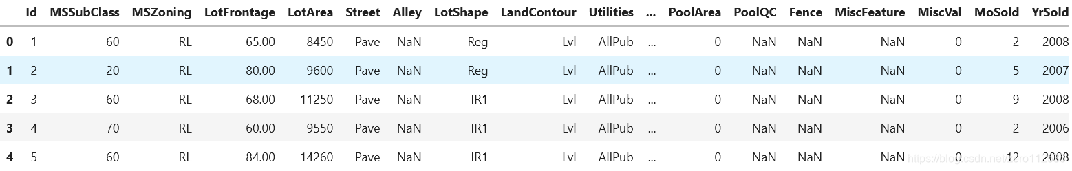
可以看到训练数据的大小是1460*81，也就是说训练数据总共有1460条，81列，其中最后一列是我们的预测目标：SalePrice。（训练数据的表格因为太长，我这里没有全部放出来）
再来看看测试数据：

test = pd.read_csv('test.csv')
print('The shape of testing data:', test.shape)
test.head()

The shape of testing data: (1459, 80)

测试数据一共是1459条，80列。
注意到Id这一列是直接从1顺次排到2919的，训练数据取的是1 ~ 1460，测试数据取的是1461 ~ 2919，说明Id和房价没有任何关系，所以直接去掉这一列：

#ID列没有用，直接删掉
train.drop('Id', axis=1, inplace=True)
test.drop('Id', axis=1, inplace=True)
print('The shape of training data:', train.shape)
print('The shape of testing data:', test.shape)

The shape of training data: (1460, 80)
The shape of testing data: (1459, 79)

去掉之后训练数据大小是146080，测试数据是145979。

目标值分析

要了解整个数据，我们首先得了解要预测的目标值，包括两方面：目标值的分布、其他特征与目标值的关系。
我们先来看看目标值的分布：

#绘制目标值分布
sns.distplot(train['SalePrice'])

明显的右偏分布，这就意味着我们之后要对目标值做一些处理，因为回归模型在正态分布的数据集上表现更好。
再看看目标值的统计值：

train['SalePrice'].describe()

count 1460.00
mean 180921.20
std 79442.50
min 34900.00
25% 129975.00
50% 163000.00
75% 214000.00
max 755000.00
Name: SalePrice, dtype: float64

最大值和均值之间差距比较大，可能会存在异常值。
这里有一个小trick：把类别特征和数字特征分离开来，在处理的时候会比较方便。

#分离数字特征和类别特征
num_features = []
cate_features = []
for col in test.columns:
    if test[col].dtype == 'object':
        cate_features.append(col)
    else:
        num_features.append(col)
print('number of numeric features:', len(num_features))
print('number of categorical features:', len(cate_features))

number of numeric features: 36
number of categorical features: 43

总共有36个数字特征，43个类别特征。
查看目标值和数字特征之间的关系（查看数字特征通常采用散点图）：

#查看数字特征与目标值的关系
plt.figure(figsize=(16, 20))
plt.subplots_adjust(hspace=0.3, wspace=0.3)
for i, feature in enumerate(num_features):
    plt.subplot(9, 4, i+1)
    sns.scatterplot(x=feature, y='SalePrice', data=train, alpha=0.5)
    plt.xlabel(feature)
    plt.ylabel('SalePrice')
plt.show()

可以看到，‘TotalBsmtSF’、'GrLiveArea’与目标值之间有明显的线性关系，那么这两个值对目标值的预测应该会有很大的帮助，这就是我们要重点关注的特征。
在类别特征中，凭直觉来看，'Neighborhood’这个特征应该是很重要的，房子的房价往往和周围的房价是差不多的，为了验证这个想法，我们来看看不同类型的’Neighborhood’房价的分布情况（查看类别特征通常采用箱线图）：

#查看‘Neighborhood’与目标值的关系
plt.figure(figsize=(16, 12))
sns.boxplot(x='Neighborhood', y='SalePrice', data=train)
plt.xlabel('Neighborhood', fontsize=14)
plt.ylabel('SalePrice', fontsize=14)
plt.xticks(rotation=90, fontsize=12)