【实验小结】cs231n assignment1 knn 部分

1. 前言

这个是斯坦福 cs231n 课程的课程作业， 在做这个课程作业的过程中， 遇到了各种问题， 通过查阅资料加以解决， 加深了对课程内容的理解， 以及熟悉了相应的python 代码实现

工程地址： https://github.com/zhyh2010/cs231n/tree/master/assignment1

2. 具体实现部分

2.1 knn 调用程序

2.1.1 简单说明

1. knn 算法原理非常简单， 我们之前也总结过一次： http://blog.csdn.net/zhyh1435589631/article/details/53875182
2. 这个算法需要 对每个输入的测试数据计算他与所有的训练集数据之间的距离 （可以是 曼哈顿距离 L1， 欧式距离 L2）， 然后挑选出其中距离最小的k个值作为 选民， 并根据他们的党派进行投票， 这是一种典型的少数服从多数的方法

2.1.2 knn 调用程序 代码分析

2.1.2.1 data_utils 载入数据集

1. 这里选用的数据集是 cifar-10 数据集 http://www.cs.toronto.edu/~kriz/cifar.html
2. 载入代码：
   输出相应的训练集和测试集数据 Xtr, Ytr, Xte, Yte

def load_CIFAR_batch(filename):
  """ load single batch of cifar """
  with open(filename, 'rb') as f:
    datadict = pickle.load(f)
    X = datadict['data']
    Y = datadict['labels']
    X = X.reshape(10000, 3, 32, 32).transpose(0,2,3,1).astype("float")
    Y = np.array(Y)
    return X, Y

def load_CIFAR10(ROOT):
  """ load all of cifar """
  xs = []
  ys = []
  for b in range(1,6):
    f = os.path.join(ROOT, 'data_batch_%d' % (b, ))
    X, Y = load_CIFAR_batch(f)
    xs.append(X)
    ys.append(Y)    
  Xtr = np.concatenate(xs)
  Ytr = np.concatenate(ys)
  del X, Y
  Xte, Yte = load_CIFAR_batch(os.path.join(ROOT, 'test_batch'))
  return Xtr, Ytr, Xte, Yte

2.1.2.2 载入数据集的调用

# Run some setup code for this notebook.

import random
import numpy as np
from cs231n.data_utils import load_CIFAR10
import matplotlib.pyplot as plt

# This is a bit of magic to make matplotlib figures appear inline in the notebook
# rather than in a new window.
%matplotlib inline
plt.rcParams['figure.figsize'] = (10.0, 8.0) # set default size of plots
plt.rcParams['image.interpolation'] = 'nearest'
plt.rcParams['image.cmap'] = 'gray'

# Some more magic so that the notebook will reload external python modules;
# see http://stackoverflow.com/questions/1907993/autoreload-of-modules-in-ipython
%load_ext autoreload
%autoreload 2

# Load the raw CIFAR-10 data.
cifar10_dir = 'cs231n/datasets/cifar-10-batches-py'
X_train, y_train, X_test, y_test = load_CIFAR10(cifar10_dir)

# As a sanity check, we print out the size of the training and test data.
print 'Training data shape: ', X_train.shape
print 'Training labels shape: ', y_train.shape
print 'Test data shape: ', X_test.shape
print 'Test labels shape: ', y_test.shape

显示结果：

Training data shape:  (50000L, 32L, 32L, 3L)
Training labels shape:  (50000L,)
Test data shape:  (10000L, 32L, 32L, 3L)
Test labels shape:  (10000L,)

2.1.2.3 显示数据集的一部分信息

# Visualize some examples from the dataset.
# We show a few examples of training images from each class.
classes = ['plane', 'car', 'bird', 'cat', 'deer', 'dog', 'frog', 'horse', 'ship', 'truck']
num_classes = len(classes)
samples_per_class = 7
for y, cls in enumerate(classes):
    idxs = np.flatnonzero(y_train == y)
    idxs = np.random.choice(idxs, samples_per_class, replace=False)
    for i, idx in enumerate(idxs):
        plt_idx = i * num_classes + y + 1
        plt.subplot(samples_per_class, num_classes, plt_idx)
        plt.imshow(X_train[idx].astype('uint8'))
        plt.axis('off')
        if i == 0:
            plt.title(cls)
plt.show()

显示结果：

2.1.2.4 调整数据集大小

# Subsample the data for more efficient code execution in this exercise
num_training = 5000
mask = range(num_training)
X_train = X_train[mask]
y_train = y_train[mask]

num_test = 500
mask = range(num_test)
X_test = X_test[mask]
y_test = y_test[mask]

# Reshape the image data into rows
X_train = np.reshape(X_train, (X_train.shape[0], -1))
X_test = np.reshape(X_test, (X_test.shape[0], -1))
print X_train.shape, X_test.shape

显示结果：

(5000L, 3072L) (500L, 3072L)

2.1.2.5 使用KNN进行训练

这段 代码训练的时间特别长。。。。。

from cs231n.classifiers import KNearestNeighbor

# Create a kNN classifier instance. 
# Remember that training a kNN classifier is a noop: 
# the Classifier simply remembers the data and does no further processing 
classifier = KNearestNeighbor()
classifier.train(X_train, y_train)

# Open cs231n/classifiers/k_nearest_neighbor.py and implement
# compute_distances_two_loops.

# Test your implementation:
dists = classifier.compute_distances_two_loops(X_test)
print dists.shape

# Now implement the function predict_labels and run the code below:
# We use k = 1 (which is Nearest Neighbor).
y_test_pred = classifier.predict_labels(dists, k=1)

# Compute and print the fraction of correctly predicted examples
num_correct = np.sum(y_test_pred == y_test)
accuracy = float(num_correct) / num_test
print 'Got %d / %d correct => accuracy: %f' % (num_correct, num_test, accuracy)

显示结果：

Got 137 / 500 correct => accuracy: 0.274000

2.1.2.6 修改 k 参数

y_test_pred = classifier.predict_labels(dists, k=5)
num_correct = np.sum(y_test_pred == y_test)
accuracy = float(num_correct) / num_test
print 'Got %d / %d correct => accuracy: %f' % (num_correct, num_test, accuracy)

显示结果：

Got 145 / 500 correct => accuracy: 0.290000

2.1.2.7 验证其他两种实现方式

结果是一致的

# Now lets speed up distance matrix computation by using partial vectorization
# with one loop. Implement the function compute_distances_one_loop and run the
# code below:
dists_one = classifier.compute_distances_one_loop(X_test)

# To ensure that our vectorized implementation is correct, we make sure that it
# agrees with the naive implementation. There are many ways to decide whether
# two matrices are similar; one of the simplest is the Frobenius norm. In case
# you haven't seen it before, the Frobenius norm of two matrices is the square
# root of the squared sum of differences of all elements; in other words, reshape
# the matrices into vectors and compute the Euclidean distance between them.
difference = np.linalg.norm(dists - dists_one, ord='fro')
print 'Difference was: %f' % (difference, )
if difference < 0.001:
  print 'Good! The distance matrices are the same'
else:
  print 'Uh-oh! The distance matrices are different'

# Now implement the fully vectorized version inside compute_distances_no_loops
# and run the code
dists_two = classifier.compute_distances_no_loops(X_test)

# check that the distance matrix agrees with the one we computed before:
difference = np.linalg.norm(dists - dists_two, ord='fro')
print 'Difference was: %f' % (difference, )
if difference < 0.001:
  print 'Good! The distance matrices are the same'
else:
  print 'Uh-oh! The distance matrices are different'

2.1.2.8 查看三种实现方法的使用时间

# Let's compare how fast the implementations are
def time_function(f, *args):
  """
  Call a function f with args and return the time (in seconds) that it took to execute.
  """
  import time
  tic = time.time()
  f(*args)
  toc = time.time()
  return toc - tic

two_loop_time = time_function(classifier.compute_distances_two_loops, X_test)
print 'Two loop version took %f seconds' % two_loop_time

one_loop_time = time_function(classifier.compute_distances_one_loop, X_test)
print 'One loop version took %f seconds' % one_loop_time

no_loop_time = time_function(classifier.compute_distances_no_loops, X_test)
print 'No loop version took %f seconds' % no_loop_time

# you should see significantly faster performance with the fully vectorized implementation

显示结果：

Two loop version took 46.657000 seconds
One loop version took 109.456000 seconds
No loop version took 1.205000 seconds

可以发现这个效率差别真不是一心半点的， 尽量使用矩阵操作少用循环

2.2.3 knn 本质实现部分 代码分析

2.2.3.1 KNearestNeighbor 类整体分析

1. 本质上， 这是一个类， 有多个成员函数构成， 用户调用的时候， 只需要调用 train 和 predict 即可得到想要的预测数据
2. 其中， compute_distances_two_loops,compute_distances_one_loop,compute_distances_no_loops分别是用来实现需要预测的数据集 X 和 原始记录的训练集 self.X_train之间的距离关系， 并通过 predict_labels 进行KNN预测

class KNearestNeighbor(object):
  """ a kNN classifier with L2 distance """

  def __init__(self):
    pass

  def train(self, X, y):
    ...

  def predict(self, X, k=1, num_loops=0):
    ...

  def compute_distances_two_loops(self, X):
    ...

  def compute_distances_one_loop(self, X):
    ...

  def compute_distances_no_loops(self, X):
    ...

  def getNormMatrix(self, x, lines_num):
    ... 

  def predict_labels(self, dists, k=1):
    ...

2.2.3.2 compute_distances_two_loops

这个函数主要通过两层 for 循环对计算测试集与训练集数据之间的欧式距离

$$d_2 (I_1, I_2) = \sqrt{\sum_{p} \left( I^p_1 - I^p_2 \right)^2}$$

def compute_distances_two_loops(self, X):
    """
    Compute the distance between each test point in X and each training point
    in self.X_train using a nested loop over both the training data and the 
    test data.

    Inputs:
    - X: A numpy array of shape (num_test, D) containing test data.

    Returns:
    - dists: A numpy array of shape (num_test, num_train) where dists[i, j]
      is the Euclidean distance between the ith test point and the jth training
      point.
    """
    num_test = X.shape[0]
    num_train = self.X_train.shape[0]
    dists = np.zeros((num_test, num_train))
    for i in xrange(num_test):
      for j in xrange(num_train):
        #####################################################################
        # TODO:                                                             #
        # Compute the l2 distance between the ith test point and the jth    #
        # training point, and store the result in dists[i, j]. You should   #
        # not use a loop over dimension.                                    #
        #####################################################################
        dists[i, j] = np.sqrt(np.dot(X[i] - self.X_train[j], X[i] - self.X_train[j]))
        #####################################################################
        #                       END OF YOUR CODE                            #
        #####################################################################
    return dists

2.2.3.3 compute_distances_one_loop

本质上这里填入的代码和 上一节中的是一致的， 只是多了一个 axis = 1 指定方向

def compute_distances_one_loop(self, X):
    """
    Compute the distance between each test point in X and each training point
    in self.X_train using a single loop over the test data.

    Input / Output: Same as compute_distances_two_loops
    """
    num_test = X.shape[0]
    num_train = self.X_train.shape[0]
    dists = np.zeros((num_test, num_train))
    for i in xrange(num_test):
      #######################################################################
      # TODO:                                                               #
      # Compute the l2 distance between the ith test point and all training #
      # points, and store the result in dists[i, :].                        #
      #######################################################################
      dists[i, :] = np.sqrt(np.sum(np.square(X[i] - self.X_train), axis = 1))
      #######################################################################
      #                         END OF YOUR CODE                            #
      #######################################################################
    return dists

2.2.3.4 compute_distances_no_loops

1. 这部分公式虽然短小， 但是需要一定的数学功底， 参考文章： http://blog.csdn.net/geekmanong/article/details/51524402
2. 我们记测试集矩阵 为 $P$ 大小为 $M \times D$ , 训练集矩阵 为 $C$ 大小为 $N \times D$
3. 记 $P_i$ 是$P$ 的第 $i$ 行， 同理 $C_j$ 是 $C$ 的 第 $j$ 行：
   $$P_i = [P_{i1} \quad P_{i2} \quad \cdots \quad P_{iD}] \\ C_j = [C_{j1} \quad C_{j2} \quad \cdots \quad C_{jD}]$$
4. 我们先来计算一下 $P_i$ 和 $C_j$ 之间的距离
   $$d(P_i, C_j) =\sqrt{(P_{i1} - P_{j1})^2 + (P_{i2} - P_{j2})^2 + \cdots + (P_{iD} - P_{jD})^2} \\ =\sqrt{(P_{i1}^2 + P_{i2}^2 + \cdots + P_{iD}^2) + (C_{j1}^2 + C_{j2}^2 + \cdots + C_{jD}^2) - 2 * (P_{i1}C_{j1} + P_{i2}C_{j2} + \cdots + P_{iD}C_{jD})} \\ =\sqrt{||P_i||^2+||C_j||^2 - 2 * P_i C_j'}$$
5. 我们可以推广得到，结果矩阵的每行元素为：
   $$Res(i) = \sqrt{(||P_i||^2 \quad ||P_i||^2 \quad \cdots ||P_i||^2) + (||C_1||^2 \quad ||C_2||^2 \quad \cdots \quad ||C_N||^2) - 2 * P_i (C_1' \quad C_2' \quad \cdots \quad C_N')} \\ =\sqrt{(||P_i||^2 \quad ||P_i||^2 \quad \cdots ||P_i||^2) + (||C_1||^2 \quad ||C_2||^2 \quad \cdots \quad ||C_N||^2) - 2 * P_iC'}$$
6. 继而， 结果矩阵为：
   $$Res = \sqrt{ \begin{pmatrix} ||P_1||^2 && ||P_1||^2 && \cdots && ||P_1||^2 \\ ||P_2||^2 && ||P_2||^2 && \cdots && ||P_2||^2 \\ \vdots && \vdots && \ddots &&\vdots\\ ||P_M||^2 && ||P_M||^2 && \cdots && ||P_M||^2 \end{pmatrix} + \begin{pmatrix} ||C_1||^2 && ||C_2||^2 && \cdots && ||C_N||^2 \\ ||C_1||^2 && ||C_2||^2 && \cdots && ||C_N||^2 \\ \vdots && \vdots && \ddots &&\vdots\\ ||C_1||^2 && ||C_2||^2 && \cdots && ||C_N||^2 \end{pmatrix} -2PC' } \\ =\sqrt{ \begin{pmatrix} ||P_1||^2 \\ ||P_2||^2 \\ \vdots \\ ||P_M||^2 \end{pmatrix}_{M\times 1} * \begin{pmatrix} 1 && 1 && \cdots && 1 \end{pmatrix}_{1 \times N} + \begin{pmatrix} 1 \\ 1 \\ \vdots \\ 1 \end{pmatrix}_{M\times 1} * \begin{pmatrix} ||C_1||^2 && ||C_2||^2 && \cdots && ||C_N||^2 \end{pmatrix}_{1 \times N} -2P_{M\times D}C'_{N\times D} }$$
7. 转换为python 代码如下：

 def compute_distances_no_loops(self, X):
    """
    Compute the distance between each test point in X and each training point
    in self.X_train using no explicit loops.

    Input / Output: Same as compute_distances_two_loops
    """
    num_test = X.shape[0]
    num_train = self.X_train.shape[0]
    dists = np.zeros((num_test, num_train)) 
    #########################################################################
    # TODO:                                                                 #
    # Compute the l2 distance between all test points and all training      #
    # points without using any explicit loops, and store the result in      #
    # dists.                                                                #
    #                                                                       #
    # You should implement this function using only basic array operations; #
    # in particular you should not use functions from scipy.                #
    #                                                                       #
    # HINT: Try to formulate the l2 distance using matrix multiplication    #
    #       and two broadcast sums.                                         #
    #########################################################################
    dists = np.sqrt(self.getNormMatrix(X, num_train).T + self.getNormMatrix(self.X_train, num_test) - 2 * np.dot(X, self.X_train.T))
    #########################################################################
    #                         END OF YOUR CODE                              #
    #########################################################################
    return dists

  def getNormMatrix(self, x, lines_num):
    """
    Get a lines_num x size(x, 1) matrix
    """ 
    return np.ones((lines_num, 1)) * np.sum(np.square(x), axis = 1) 

从最终得到的结果看， 这个推导的结果运行速度是最快的

2.2.3.5 predict_labels

根据计算得到的距离关系， 挑选 K 个数据组成选民， 进行党派选举

def predict_labels(self, dists, k=1):
    """
    Given a matrix of distances between test points and training points,
    predict a label for each test point.

    Inputs:
    - dists: A numpy array of shape (num_test, num_train) where dists[i, j]
      gives the distance betwen the ith test point and the jth training point.

    Returns:
    - y: A numpy array of shape (num_test,) containing predicted labels for the
      test data, where y[i] is the predicted label for the test point X[i].  
    """
    num_test = dists.shape[0]
    y_pred = np.zeros(num_test)
    for i in xrange(num_test):
      # A list of length k storing the labels of the k nearest neighbors to
      # the ith test point.
      closest_y = []
      #########################################################################
      # TODO:                                                                 #
      # Use the distance matrix to find the k nearest neighbors of the ith    #
      # testing point, and use self.y_train to find the labels of these       #
      # neighbors. Store these labels in closest_y.                           #
      # Hint: Look up the function numpy.argsort.                             #
      #########################################################################
      kids = np.argsort(dists[i])
      closest_y = self.y_train[kids[:k]]
      #########################################################################
      # TODO:                                                                 #
      # Now that you have found the labels of the k nearest neighbors, you    #
      # need to find the most common label in the list closest_y of labels.   #
      # Store this label in y_pred[i]. Break ties by choosing the smaller     #
      # label.                                                                #
      #########################################################################
      count = 0
      label = 0
      for j in closest_y:
         tmp = 0
         for kk in closest_y:
            tmp += (kk == j)
         if tmp > count:
            count = tmp
            label = j
      y_pred[i] = label
      #y_pred[i] = np.argmax(np.bincount(closest_y))
      #########################################################################
      #                           END OF YOUR CODE                            # 
      #########################################################################

    return y_pred

2.2.3.6 predict

1. 这里主要做了两个步骤：
   
   1. 计算欧式距离
   2. KNN 统计预测信息

def predict(self, X, k=1, num_loops=0):
    """
    Predict labels for test data using this classifier.

    Inputs:
    - X: A numpy array of shape (num_test, D) containing test data consisting
         of num_test samples each of dimension D.
    - k: The number of nearest neighbors that vote for the predicted labels.
    - num_loops: Determines which implementation to use to compute distances
      between training points and testing points.

    Returns:
    - y: A numpy array of shape (num_test,) containing predicted labels for the
      test data, where y[i] is the predicted label for the test point X[i].  
    """
    if num_loops == 0:
      dists = self.compute_distances_no_loops(X)
    elif num_loops == 1:
      dists = self.compute_distances_one_loop(X)
    elif num_loops == 2:
      dists = self.compute_distances_two_loops(X)
    else:
      raise ValueError('Invalid value %d for num_loops' % num_loops)

    return self.predict_labels(dists, k=k)

2.2.4 cross-validation 代码分析

1. 交叉验证实际上是将数据的训练集进行拆分， 分成多个组， 构成多个训练和测试集， 来筛选较好的超参数
2. 
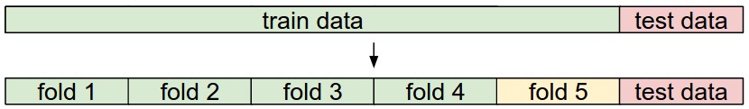
3. 如图所示， 可以分为 5组数据， （分别将 fold 1, 2 .. 5 作为验证集， 将剩余的数据作为训练集， 训练得到超参数）

2.2.4.1 筛选不同的k

num_folds = 5
k_choices = [1, 3, 5, 8, 10, 12, 15, 20, 50, 100]

X_train_folds = []
y_train_folds = []
################################################################################
# TODO:                                                                        #
# Split up the training data into folds. After splitting, X_train_folds and    #
# y_train_folds should each be lists of length num_folds, where                #
# y_train_folds[i] is the label vector for the points in X_train_folds[i].     #
# Hint: Look up the numpy array_split function.                                #
################################################################################
X_train_folds = np.array_split(X_train, num_folds)
y_train_folds = np.array_split(y_train, num_folds)


################################################################################
#                                 END OF YOUR CODE                             #
################################################################################

# A dictionary holding the accuracies for different values of k that we find
# when running cross-validation. After running cross-validation,
# k_to_accuracies[k] should be a list of length num_folds giving the different
# accuracy values that we found when using that value of k.
k_to_accuracies = {}


################################################################################
# TODO:                                                                        #
# Perform k-fold cross validation to find the best value of k. For each        #
# possible value of k, run the k-nearest-neighbor algorithm num_folds times,   #
# where in each case you use all but one of the folds as training data and the #
# last fold as a validation set. Store the accuracies for all fold and all     #
# values of k in the k_to_accuracies dictionary.                               #
################################################################################
for k in k_choices:
    k_to_accuracies[k] = np.zeros(num_folds)
    for i in range(num_folds):
        Xtr = np.array(X_train_folds[:i] + X_train_folds[i+1:])
        ytr = np.array(y_train_folds[:i] + y_train_folds[i+1:])
        Xte = np.array(X_train_folds[i])
        yte = np.array(y_train_folds[i])     

        Xtr = np.reshape(Xtr, (X_train.shape[0] * 4 / 5, -1))
        ytr = np.reshape(ytr, (y_train.shape[0] * 4 / 5, -1))
        Xte = np.reshape(Xte, (X_train.shape[0] / 5, -1))
        yte = np.reshape(yte, (y_train.shape[0] / 5, -1))

        classifier.train(Xtr, ytr)
        yte_pred = classifier.predict(Xte, k)
        yte_pred = np.reshape(yte_pred, (yte_pred.shape[0], -1))
        num_correct = np.sum(yte_pred == yte)
        accuracy = float(num_correct) / len(yte)
        k_to_accuracies[k][i] = accuracy

################################################################################
#                                 END OF YOUR CODE                             #
################################################################################

# Print out the computed accuracies
for k in sorted(k_to_accuracies):
    for accuracy in k_to_accuracies[k]:
        print 'k = %d, accuracy = %f' % (k, accuracy)

显示结果：

k = 1, accuracy = 0.263000
k = 1, accuracy = 0.257000
k = 1, accuracy = 0.264000
k = 1, accuracy = 0.278000
k = 1, accuracy = 0.266000
k = 3, accuracy = 0.257000
k = 3, accuracy = 0.263000
k = 3, accuracy = 0.273000
k = 3, accuracy = 0.282000
k = 3, accuracy = 0.270000
k = 5, accuracy = 0.265000
k = 5, accuracy = 0.275000
k = 5, accuracy = 0.295000
k = 5, accuracy = 0.298000
k = 5, accuracy = 0.284000
k = 8, accuracy = 0.272000
k = 8, accuracy = 0.295000
k = 8, accuracy = 0.284000
k = 8, accuracy = 0.298000
k = 8, accuracy = 0.290000
k = 10, accuracy = 0.272000
k = 10, accuracy = 0.303000
k = 10, accuracy = 0.289000
k = 10, accuracy = 0.292000
k = 10, accuracy = 0.285000
k = 12, accuracy = 0.271000
k = 12, accuracy = 0.305000
k = 12, accuracy = 0.285000
k = 12, accuracy = 0.289000
k = 12, accuracy = 0.281000
k = 15, accuracy = 0.260000
k = 15, accuracy = 0.302000
k = 15, accuracy = 0.292000
k = 15, accuracy = 0.292000
k = 15, accuracy = 0.285000
k = 20, accuracy = 0.268000
k = 20, accuracy = 0.293000
k = 20, accuracy = 0.291000
k = 20, accuracy = 0.287000
k = 20, accuracy = 0.286000
k = 50, accuracy = 0.273000
k = 50, accuracy = 0.291000
k = 50, accuracy = 0.274000
k = 50, accuracy = 0.267000
k = 50, accuracy = 0.273000
k = 100, accuracy = 0.261000
k = 100, accuracy = 0.272000
k = 100, accuracy = 0.267000
k = 100, accuracy = 0.260000
k = 100, accuracy = 0.267000

2.2.4.2 图形化显示

# plot the raw observations
for k in k_choices:
  accuracies = k_to_accuracies[k]
  plt.scatter([k] * len(accuracies), accuracies)

# plot the trend line with error bars that correspond to standard deviation
accuracies_mean = np.array([np.mean(v) for k,v in sorted(k_to_accuracies.items())])
accuracies_std = np.array([np.std(v) for k,v in sorted(k_to_accuracies.items())])
plt.errorbar(k_choices, accuracies_mean, yerr=accuracies_std)
plt.title('Cross-validation on k')
plt.xlabel('k')
plt.ylabel('Cross-validation accuracy')
plt.show()

显示结果：

2.2.4.3 选取最好的k 进行训练

# Based on the cross-validation results above, choose the best value for k,   
# retrain the classifier using all the training data, and test it on the test
# data. You should be able to get above 28% accuracy on the test data.
best_k = 8

classifier = KNearestNeighbor()
classifier.train(X_train, y_train)
y_test_pred = classifier.predict(X_test, k=best_k)

# Compute and display the accuracy
num_correct = np.sum(y_test_pred == y_test)
accuracy = float(num_correct) / num_test
print 'Got %d / %d correct => accuracy: %f' % (num_correct, num_test, accuracy)

显示结果：

Got 147 / 500 correct => accuracy: 0.294000

可以发现， 即使是最好情况下， KNN算法的识别准确率也只有30%， 因而， 一般不用来做图像分类

3. 参考资料

1. 寒老师博客 http://blog.csdn.net/han_xiaoyang/article/details/49949535
2. cs231n 课程主页 http://vision.stanford.edu/teaching/cs231n/syllabus.html
3. github 主页 http://cs231n.github.io/
4. http://www.cnblogs.com/daihengchen/p/5754383.html
5. https://docs.scipy.org/doc/numpy/reference/generated/numpy.sqrt.html
6. https://docs.scipy.org/doc/numpy-1.10.1/reference/generated/numpy.sum.html
7. https://docs.scipy.org/doc/numpy/reference/generated/numpy.ndarray.shape.html
8. https://docs.scipy.org/doc/numpy/reference/generated/numpy.reshape.html
9. enumerate ： http://blog.chinaunix.net/uid-27040911-id-3429751.html
10. https://docs.scipy.org/doc/numpy-dev/reference/generated/numpy.random.choice.html
11. https://docs.scipy.org/doc/numpy/reference/generated/numpy.flatnonzero.html
12. https://docs.scipy.org/doc/numpy/reference/generated/numpy.sum.html
13. https://docs.scipy.org/doc/numpy/reference/generated/numpy.concatenate.html
14. https://docs.scipy.org/doc/numpy/reference/generated/numpy.ones.html
15. https://docs.scipy.org/doc/numpy/reference/generated/numpy.count_nonzero.html#numpy.count_nonzero
16. https://docs.scipy.org/doc/numpy/reference/generated/numpy.argsort.html
17. https://docs.scipy.org/doc/numpy/reference/generated/numpy.bincount.html
18. https://docs.scipy.org/doc/numpy/reference/generated/numpy.multiply.html
19. https://docs.scipy.org/doc/numpy/reference/generated/numpy.dot.html
20. https://docs.scipy.org/doc/numpy/reference/generated/numpy.array_split.html