VGG16神经网络模型复现

VGG网络是在2014年由牛津大学著名研究组VGG (Visual Geometry Group) 提出，斩获该年ImageNet竞赛中 Localization Task (定位任务) 第一名 和 Classification Task (分类任务) 第二名。原论文名称是《Very Deep Convolutional Networks For Large-Scale Image Recognition》，在原论文中给出了一系列VGG模型的配置，下面这幅图是VGG16模型的结构简图。

该网络中的亮点： 通过堆叠多个3x3的卷积核来替代大尺度卷积核（在拥有相同感受野的前提下能够减少所需参数）。

论文中提到，可以通过堆叠两层3x3的卷积核替代一层5x5的卷积核，堆叠三层3x3的卷积核替代一层7x7的卷积核。下面给出一个示例：使用7x7卷积核所需参数，与堆叠三个3x3卷积核所需参数(假设输入输出特征矩阵深度channel都为C)
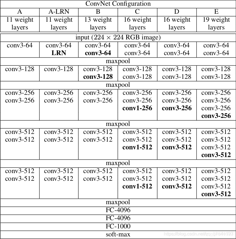
VGG模型所有层参数表：

CNN感受野：在卷积神经网络中，决定某一层输出 结果中一个元素所对应的输入层的区域大小，被称作感受野(receptive field)。通俗 的解释是，输出feature map上的一个单元 对应输入层上的区域大小。
感受野计算公式：
F (i) = (F (i +1) - 1)*Stride + Ksize
F(i)为第i层感受野， Stride为第i层的步距， Ksize为卷积核或池化核尺寸

VGG16模型框架tensor版本

from tensorflow.keras import layers, models, Model, Sequential
#3、
#定义VGG函数，传入参数feature,图片高、宽、种类
def VGG(feature, im_height=224, im_width=224, class_num=1000):
    # tensorflow中的tensor通道排序是NHWC
    input_image = layers.Input(shape=(im_height, im_width, 3), dtype="float32")
    # 1、提取特征网络结构
    x = feature(input_image)
    #2、分类网络结构
    x = layers.Flatten()(x)#展平处理，得到一维向量
    x = layers.Dropout(rate=0.5)(x)#将50%的神经元随机失活，减少过拟合
    x = layers.Dense(2048, activation='relu')(x)#全连接层1
    x = layers.Dropout(rate=0.5)(x)#将50%的神经元随机失活，减少过拟合
    x = layers.Dense(2048, activation='relu')(x)#全连接层2
    x = layers.Dense(class_num)(x)#全连接层3
    output = layers.Softmax()(x)#输出类别概率分布
    model = models.Model(inputs=input_image, outputs=output)#定义models.Model类，创建神经网络模型
    return model
#2、
#提取特征网络结构，定义features函数
def features(cfg):
    feature_layers = []#feature_layers 定义一个空列表，用来存储网络特征结构
    for v in cfg:      #for循环遍历
        if v == "M":   #判断是否为“M”
            feature_layers.append(layers.MaxPool2D(pool_size=2, strides=2)) #池化核大小为2，步长为2
        else:
            conv2d = layers.Conv2D(v, kernel_size=3, padding="SAME", activation="relu")#卷积核大小为3，步长为1
            feature_layers.append(conv2d)
    return Sequential(feature_layers, name="feature")# 跳出当前循环

#1、
#配置列表，字典(键值)
cfgs = {
    'vgg11': [64, 'M', 128, 'M', 256, 256, 'M', 512, 512, 'M', 512, 512, 'M'],
    'vgg13': [64, 64, 'M', 128, 128, 'M', 256, 256, 'M', 512, 512, 'M', 512, 512, 'M'],
    'vgg16': [64, 64, 'M', 128, 128, 'M', 256, 256, 256, 'M', 512, 512, 512, 'M', 512, 512, 512, 'M'],
    'vgg19': [64, 64, 'M', 128, 128, 'M', 256, 256, 256, 256, 'M', 512, 512, 512, 512, 'M', 512, 512, 512, 512, 'M'],
}

#实例化vgg网络模型
def vgg(model_name="vgg16", im_height=224, im_width=224, class_num=1000):
    try:
        cfg = cfgs[model_name]#传入配置列表
    except:
        print("Warning: model number {} not in cfgs dict!".format(model_name))
        exit(-1)
    model = VGG(features(cfg), im_height=im_height, im_width=im_width, class_num=class_num)
    return model

# model = vgg(model_name='vgg16')

数据标签:“0”: “daisy”, “1”: “dandelion”, “2”: “roses”,“3”: “sunflowers”, “4”: “tulips”

在花分类（flower_photos）数据集的测试结果：
（1）在cpu上训练

（2）在GPU上训练

实验结果表明在gpu上训练 一个epoch用了38s，在cpu上训练 一个epoch平均用了12s，这表明用gpu多进程训练神经网络时间更快。gpu上训练的准确度为74.90比cpu上训练的准确度74.59更高。