吴恩达机器学习作业8 ：Anomaly Detection and Recommender Systems python 实现

一、异常检测

例子1：二维数据的异常检测

1.数据可视化

data = scio.loadmat(r'ex8data1.mat')
X = data['X']
Xval = data['Xval']
yval = data['yval']

# 数据可视化
plt.scatter(X[:, 0], X[:, 1], c='b', marker='x')
plt.show()

结果：

2.正态分布图

mu, sigma2 = estimate_gaussian(X)
visualize_fit(X, mu, sigma2)

可视化函数：

import numpy as np
import matplotlib.pyplot as plt
from multivariateGaussian import multi_variate_gaussian


def visualize_fit(x, mu, sigma2):

    xx, yy = np.meshgrid(np.linspace(0, 35, 200), np.linspace(0, 35, 200))
    Z = multi_variate_gaussian(np.c_[xx.flatten(), yy.flatten()], mu, sigma2)
    Z = Z.reshape(xx.shape[0], xx.shape[1])

    plt.scatter(x[:, 0], x[:, 1])
    lev = 10 ** np.arange(-20, 0, 3).astype(np.float)
    plt.contour(xx, yy, Z, levels=lev)
    plt.show()

结果：

3. 选择判断异常与否的临界点ε

选择实现：

1. 根据训练集求出n个特征各自的的平均值mu与方差σ^2

2. 求出交叉验证集每个example的 总p(x)

   注意这里的 总p(x) 有两种计算方法：

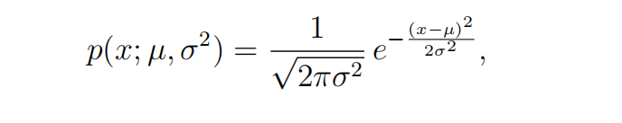
第一种：一个example有n个特征，用下面的公式计算每一个特征的p(x)然后全部相乘得到总p(x)。

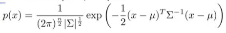
第二种 ：加入协方差矩阵进行计算。

总p(x) 的实现：

import numpy as np

# ======================== 版本1 ===========================================
# def multi_variate_gaussian(x, mu, sigma2):
#
#     p = 1 / np.square(2 * np.pi * sigma2) * \
#         np.exp(-np.power(x-mu, 2) / (2 * sigma2))
#
#     return np.multiply(p[:, 0], p[:, 1])

# =========================== 版本2 ==========================================


def multi_variate_gaussian(X, mu, sigma2):
    k = mu.size
    if sigma2.ndim == 1 or (sigma2.ndim == 2 and (sigma2.shape[1] == 1 or sigma2.shape[0] == 1)):
        sigma2 = np.diag(sigma2)

    x = X - mu
    p = (2 * np.pi) ** (-k / 2) * np.linalg.det(sigma2) ** (-0.5) * np.exp(-0.5*np.sum(np.dot(x, np.linalg.pinv(sigma2)) * x, axis=1))

    return p

选择函数的实现：

import numpy as np


def select_threshold(yval, p):

    bestEpsilon = 0
    bestF1 = 0
    F1 = 0

    stepsize = (p.max() - p.min()) / 1000
    for epsilon in np.arange(p.min(), p.max(), stepsize):

        pred = np.where(p < epsilon, 1, 0).reshape(yval.shape[0], yval.shape[1])

        tp = np.sum(np.multiply(pred, yval))
        fp = np.sum(np.where(pred > yval, 1, 0))
        fn = np.sum(np.where(pred < yval, 1, 0))

        prec = tp / (tp + fp)
        rec = tp / (tp + fn)

        F1 = (2 * prec * rec) / (prec + rec)

        if F1 > bestF1:

            bestF1 = F1
            bestEpsilon = epsilon

    return bestEpsilon

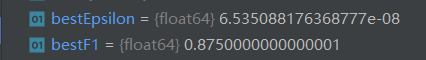
两种计算方式结果：

第一种：

第二种：

可以看见，从F1来衡量这两种算法，结果是一样的。不同的只是最终选择ε的值不同。

例子2：高维数据的异常检测

# 加载数据
data = scio.loadmat(r'ex8data2.mat')
X = data['X']
Xval = data['Xval']
yval = data['yval']

mu, sigma2 = estimate_gaussian(X)
p = multi_variate_gaussian(Xval, mu, sigma2)
best_epsilon = select_threshold(yval, p)

结果：

二、电影推荐系统

代价函数：

import numpy as np


def cofi_costfunc(com_mat, R, Y, num_movies, num_users,num_feature, mylambda):

    X = com_mat[0:num_movies*num_feature].reshape(num_movies, num_feature)
    Theta = com_mat[num_movies*num_feature:].reshape(num_users , num_feature)

    pred = np.dot(X, Theta.T)
    cost = np.sum(np.multiply(pred - Y, R)) / 2 + \
           (mylambda / 2) * np.sum(np.power(Theta[1:, 1:], 2)) + (mylambda / 2) * np.sum(np.power(X[1:, 1:], 2))

    return cost

梯度下降函数：

import numpy as np


def gradinet(com_mat, R, Y, num_movies, num_users, num_feature, mylambda):

    X = com_mat[0:num_movies * num_feature].reshape(num_movies, num_feature)
    Theta = com_mat[num_movies * num_feature:].reshape(num_users, num_feature)

    error = np.multiply(np.dot(X, Theta.T) - Y, R)

    grad_Theta = np.dot(error.T, X) + Theta * mylambda
    grad_X = np.dot(error, Theta) + X * mylambda

    return np.r_[grad_X.flatten(), grad_Theta.flatten()]

训练过程：（主函数）

# ========================  练习二 part1 ======================================
# 加载数据
data1 = scio.loadmat(r'ex8_movies.mat')
Y = data1['Y']
R = data1['R']

data2 = scio.loadmat(r'ex8_movieParams.mat')
X = data2['X']
Theta = data2['Theta']
num_users = data2['num_users'][0, 0]
num_movies = data2['num_movies'][0, 0]
num_features = data2['num_features'][0, 0]

# 初始化自己的序列
my_ratings = np.zeros(num_movies)

# 电影评分
my_ratings[0] = 4
my_ratings[97] = 2
my_ratings[6] = 3
my_ratings[11] = 5
my_ratings[53] = 4
my_ratings[63] = 5
my_ratings[66] = 3
my_ratings[68] = 5
my_ratings[183] = 4
my_ratings[225] = 5
my_ratings[354] = 5

# 加载电影名字
movies_list = load_movie_list()

# for i in range(len(my_ratings)):
#     if my_ratings[i] > 0:
#         print('Rated {} for {}'.format(my_ratings[i], movies_list[i]))

# 在原始的Y中加入一列自己对电影的评分，R中对应加入一列向量判断是否评分
Y = np.c_[my_ratings, Y]
R = np.c_[my_ratings != 0, R]

# 初始化X， Theta
initia_X = np.random.randn(num_movies, num_features)
initia_Theta = np.random.randn(num_users + 1, num_features)

mat = np.r_[initia_X.flatten(), initia_Theta.flatten()]
mylambda = 1.5

# 标准化函数
Ynorm, Ymean = normalize_ratings(Y, R)

# 最小化函数
result = opt.minimize(fun=cofi_costfunc, x0=mat,
                      args=(R, Ynorm, num_movies, num_users + 1, num_features, mylambda), method='TNC', jac=gradinet)

print(result)
res_mat = result.x
res_X = res_mat[0:num_movies * num_features].reshape(num_movies, num_features)
res_Theta = res_mat[num_movies * num_features:].reshape(num_users + 1, num_features)

# 预测分数
res_Y = np.dot(res_X, res_Theta.T)
my_predictions = res_Y[:, 0] + Ymean

加载电影名字 txt 文件的函数：

def load_movie_list():
    movie_list = []
    with open(r'movie_ids.txt', 'r', encoding='ISO-8859-1') as f:
        lines = f.readlines()
        for line in lines:
            idx, *movie_name = line.split(' ')
            # join在每行元素之间加入空格成为用空格连接的一个元素
            # rstrip（）除去原txt字符后面的空格（换行符号）
            movie_list.append(' '.join(movie_name).rstrip())

    return movie_list

训练结果：

预测结果：