


怎么找到使成本函数J达到最小值的一组w和b呢——有专门一套方法,叫梯度下降法
本次记录:梯度下降法以及线性回归中的梯度下降
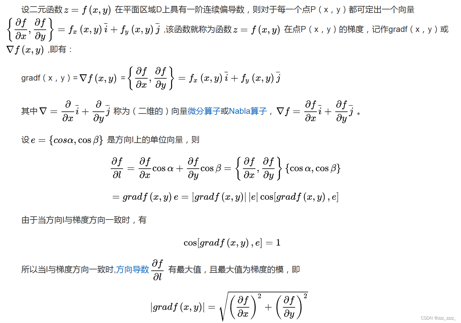
梯度下降法开始之前,要明白什么是梯度
上面是百度上的截图
也就是说有一个f(x,y)的函数,定义grad f(x,y)=f(x,y)=(
,
) 【这是定义,也就是规定是这样的,既已规定,规定就不用深究啦】值得深究的是它作为一个向量,方向有什么意义,大小又代表什么?为什么沿这个梯度变化率最大?也就是最陡?
这与方向导数的计算有关,具体写在下面: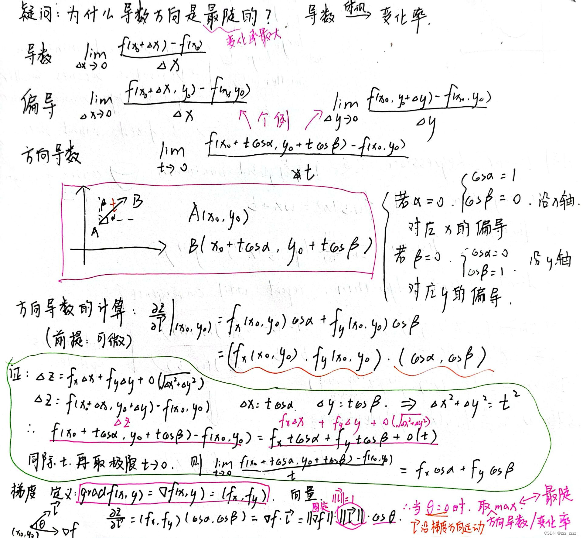
高中就知道,某一点的导数就是斜率,其绝对值的大小反映了这一点的变化快慢。在三维空间中的函数,二个自变量x和y,图形呈一个面状(曲面或者平面),在某一点它能朝各个方向运动(360度)。由此,提出了方向导数的概念。但一开始接触以及接触更多的是沿x方向运动的变化率以及沿y方向运动的变化率,即和
。方向导数的前提是可微,由此可以推出它的计算公式,可以写成两个向量相乘的形式(如上图中),角度
和
分别是运动方向和x轴正方向与y轴正方向的夹角。向量相乘可以写成模*模*夹角的形式。由此可知,要使得这个方向导数取得最大值,就要沿着这点的梯度方向运动,且变化率最大值为梯度的大小。
以上介绍的是梯度的相关内容(关键是要知道沿着梯度方向,变化率是最大的)
下面再看梯度下降法是干什么的?
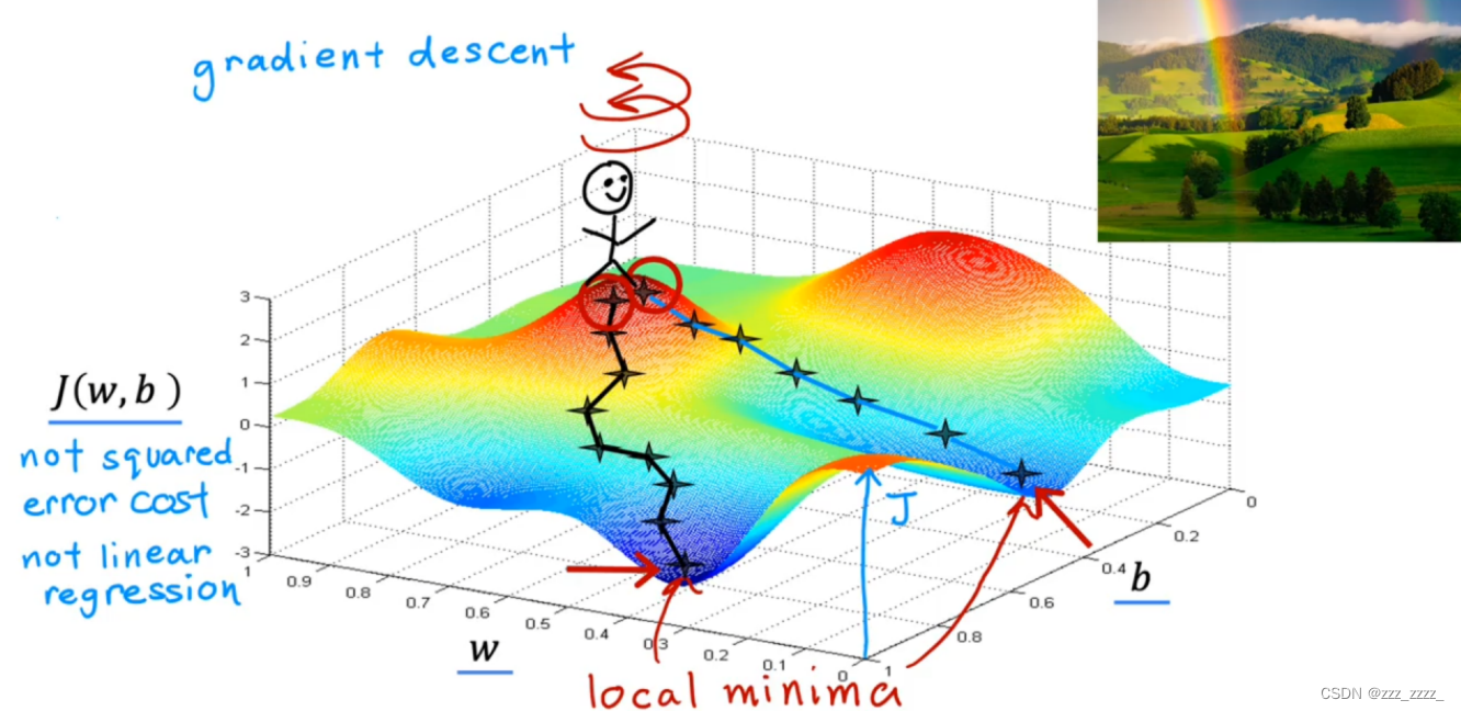
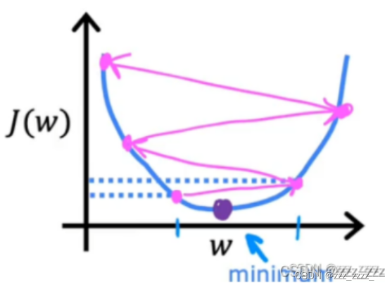
先不管线性回归的成本函数(一个相对简单的碗状/吊床状的曲面),先看一个更复杂的曲面(就像一个个丘陵)
现有一个小人站在丘陵上的某一位置上,在这个位置上他旋转360度,选择了一个最陡的方向(这个方向的变化率最大,也就是这一点的梯度方向)迈出了一小步(a baby step)。到达一个新位置后,重复上述,一直到他到达一个局部最小值点附近。也就是,这个小人沿着到达每一点的梯度方向(严格来说是梯度的反方向)走,最终会走到一个局部最小值点。
如果这个曲面有不止一个的局部最小值点,从不同的起点出来,最终到达的局部最小值也可能不一样(如图中的两个路线)。
这是对于梯度下降法比较直观的理解。
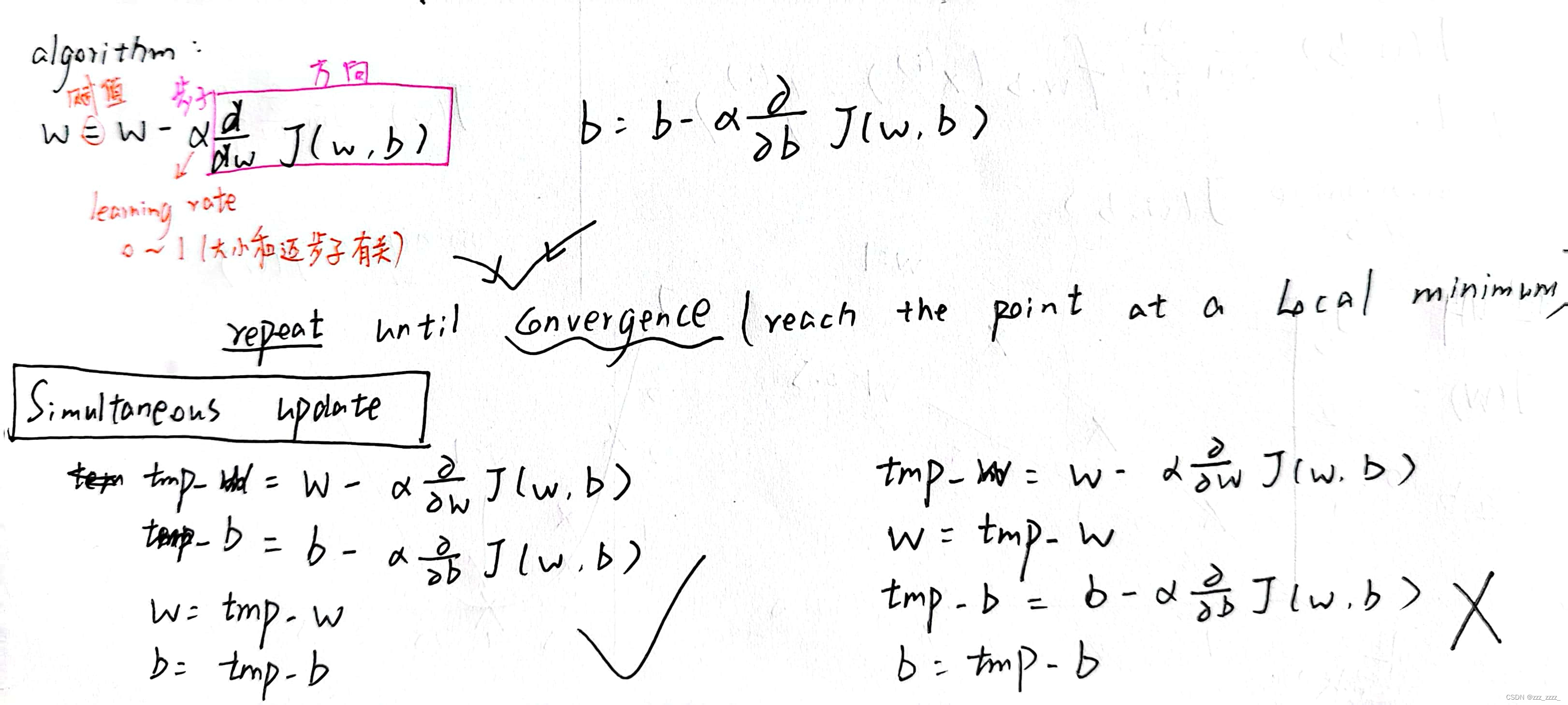
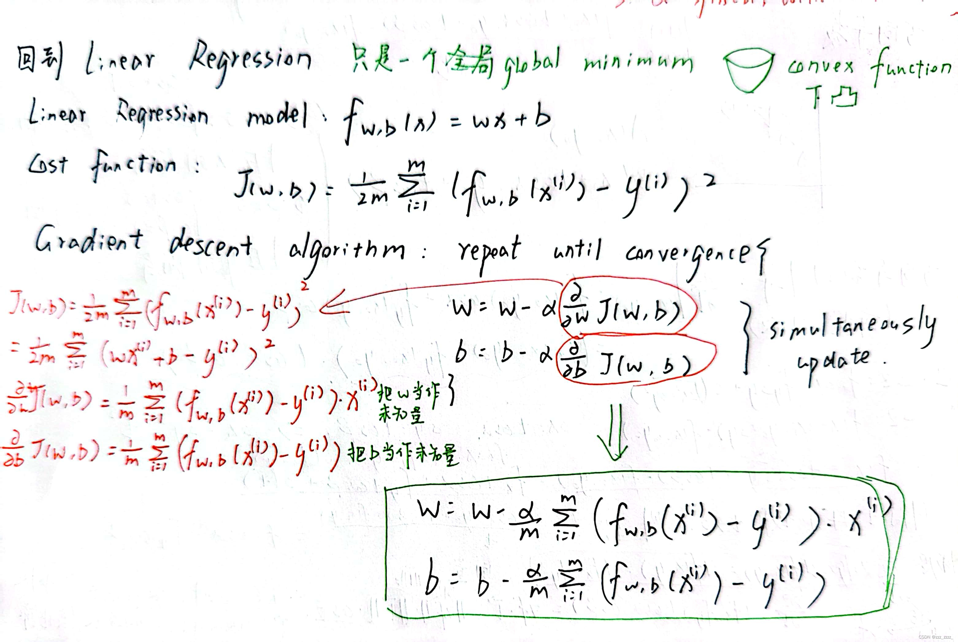
梯度下降法的算法:
对应PPT如下: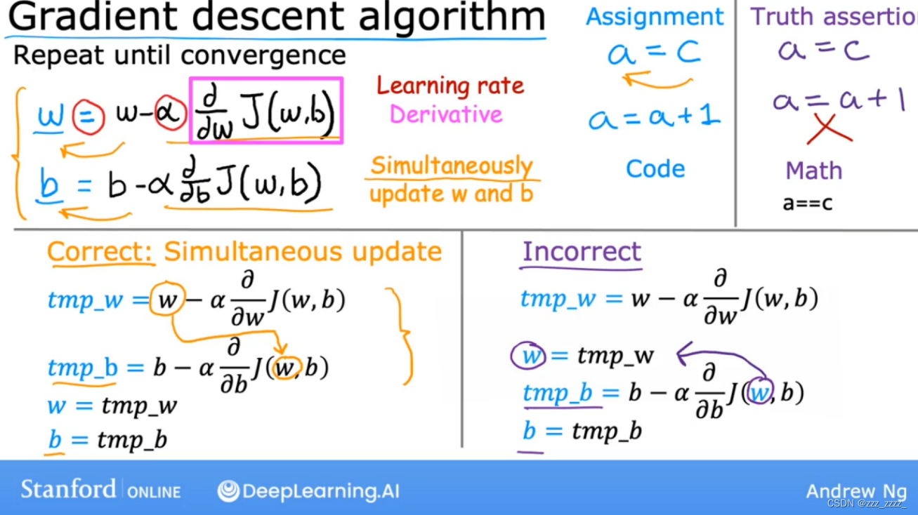
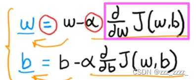
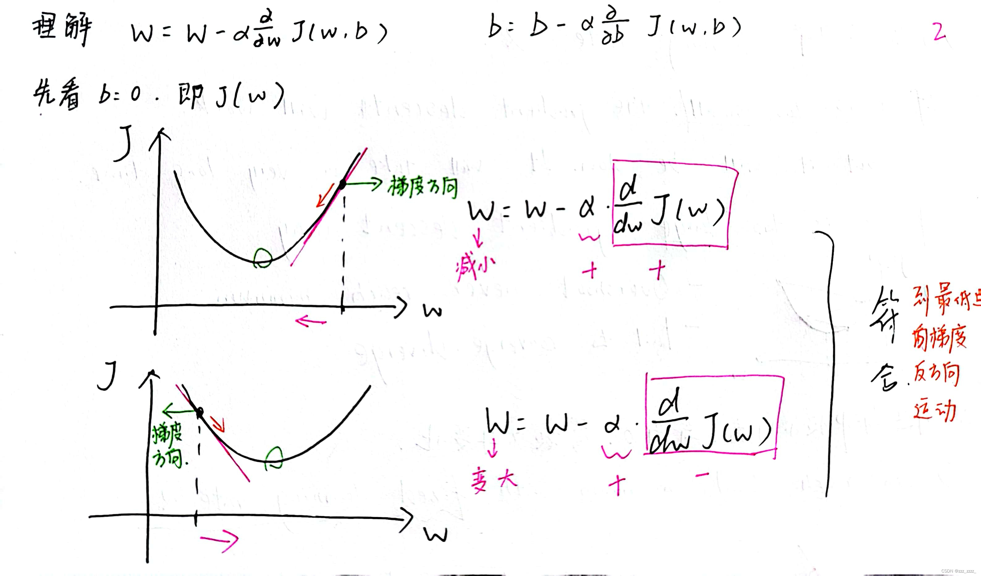
这两个式子是关键,这里可以将偏导理解为选定一个方向,(
0)理解为步长(也许不太准确但方便理解)至于为什么是减法,因为要沿着梯度的反方向走才行,见下图:
还有一点,是关于,它叫学习率(learning rate),下面这页PPT可以很好的解释它:
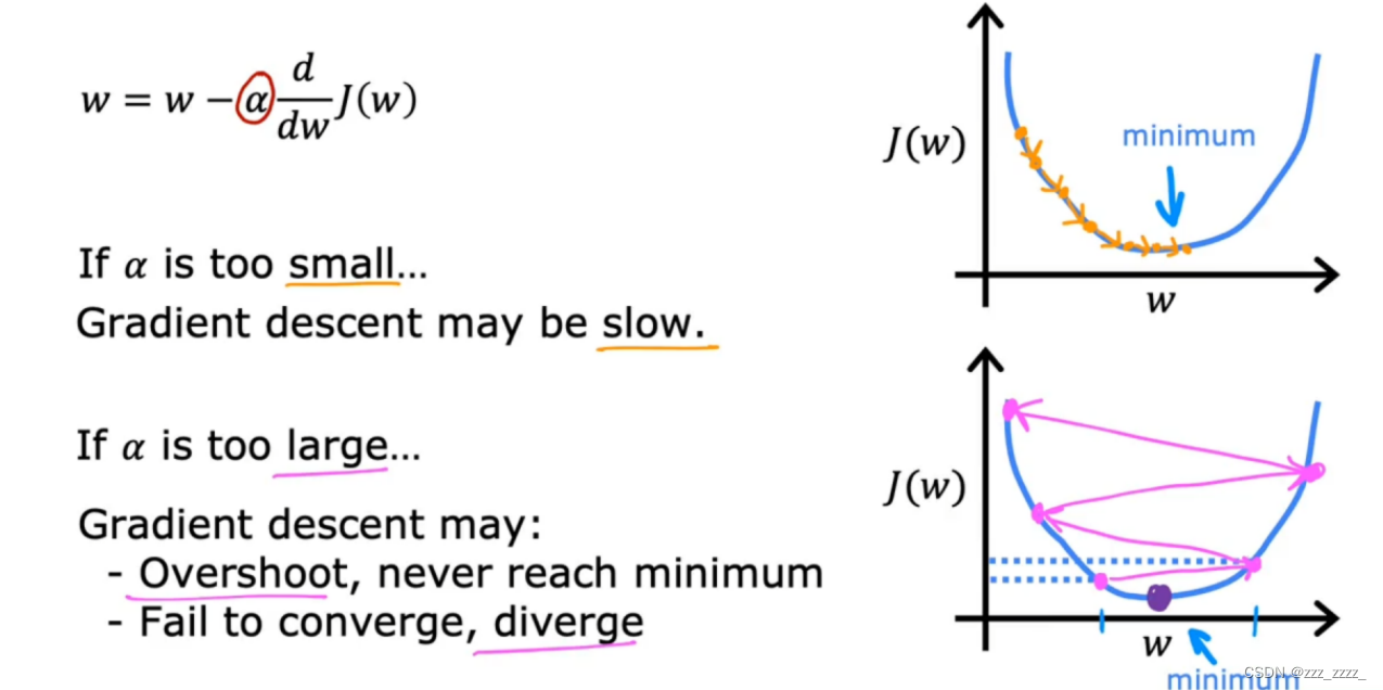
除了不能过小也不能过大外,它的值是固定的:
当到达极小值附近时,导数会变小(直观说,会越来越平坦),学习率不需要变化,它的移动的步子就会变小。直到到达极小值点,导为0,不用在移动步子了。这也解释了梯度下降中的下降,导数值在逐渐减小。
回到线性回归(Linear Regression)
下面是相关代码:
1.需要用到的库和模块
import math, copy
import numpy as np
import matplotlib.pyplot as plt
plt.style.use('./deeplearning.mplstyle')
from lab_utils_uni import plt_house_x, plt_contour_wgrad, plt_divergence, plt_gradients
2.训练样本集
# Load our data set
x_train = np.array([1.0, 2.0])   #features
y_train = np.array([300.0, 500.0])   #target value
3.计算成本的函数
#Function to calculate the cost
def compute_cost(x, y, w, b):

    m = x.shape[0]
    cost = 0

    for i in range(m):
        f_wb = w * x[i] + b
        cost = cost + (f_wb - y[i])**2
    total_cost = 1 / (2 * m) * cost

    return total_cost
4.计算偏导的函数
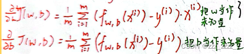
def compute_gradient(x, y, w, b):
    """
    Computes the gradient for linear regression
    Args:
      x (ndarray (m,)): Data, m examples
      y (ndarray (m,)): target values
      w,b (scalar)    : model parameters
    Returns
      dj_dw (scalar): The gradient of the cost w.r.t. the parameters w
      dj_db (scalar): The gradient of the cost w.r.t. the parameter b
     """

    # Number of training examples
    m = x.shape[0]
    dj_dw = 0
    dj_db = 0

    for i in range(m):
        f_wb = w * x[i] + b
        dj_dw_i = (f_wb - y[i]) * x[i]
        dj_db_i = f_wb - y[i]
        dj_db += dj_db_i
        dj_dw += dj_dw_i
    dj_dw = dj_dw / m
    dj_db = dj_db / m

    return dj_dw, dj_db
5.成本函数以及梯度分布图
plt_gradients(x_train,y_train, compute_cost, compute_gradient)
plt.show()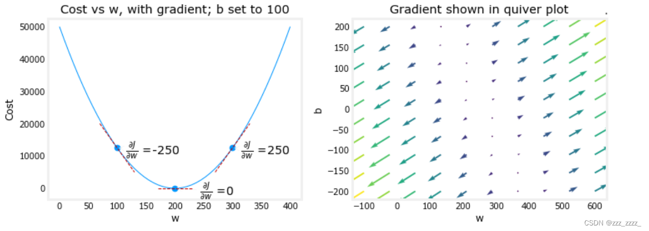
从这上面右图中可以看出要沿着梯度的反方向走
6.实现梯度下降的函数及其调用
def gradient_descent(x, y, w_in, b_in, alpha, num_iters, cost_function, gradient_function):
    """
    Performs gradient descent to fit w,b. Updates w,b by taking
    num_iters gradient steps with learning rate alpha

    Args:
      x (ndarray (m,))  : Data, m examples
      y (ndarray (m,))  : target values
      w_in,b_in (scalar): initial values of model parameters
      alpha (float):     Learning rate
      num_iters (int):   number of iterations to run gradient descent
      cost_function:     function to call to produce cost
      gradient_function: function to call to produce gradient

    Returns:
      w (scalar): Updated value of parameter after running gradient descent
      b (scalar): Updated value of parameter after running gradient descent
      J_history (List): History of cost values
      p_history (list): History of parameters [w,b]
      """

    w = copy.deepcopy(w_in) # avoid modifying global w_in
    # An array to store cost J and w's at each iteration primarily for graphing later
    J_history = []
    p_history = []
    b = b_in  #初始的b
    w = w_in  #初始的w

    for i in range(num_iters):
        # Calculate the gradient and update the parameters using gradient_function
        dj_dw, dj_db = gradient_function(x, y, w , b)     #计算两个偏导

        # Update Parameters using equation (3) above
        #代入公式计算新的w和b
        b = b - alpha * dj_db
        w = w - alpha * dj_dw

        # Save cost J at each iteration
        if i<100000:      # prevent resource exhaustion
            J_history.append( cost_function(x, y, w , b))  #存入新位置的成本
            p_history.append([w,b])   #存入新位置的一组w和b
        # Print cost every at intervals 10 times or as many iterations if < 10
        if i% math.ceil(num_iters/10) == 0:
            print(f"Iteration {i:4}: Cost {J_history[-1]:0.2e} ",
                  f"dj_dw: {dj_dw: 0.3e}, dj_db: {dj_db: 0.3e}  ",
                  f"w: {w: 0.3e}, b:{b: 0.5e}")  #并不是每一次调整w和b的值都输出一次,每1000次调整输出一次值

    return w, b, J_history, p_history #return w and J,w history for graphing
下面是调用上面的函数
# initialize parameters
w_init = 0
b_init = 0
# some gradient descent settings
iterations = 10000
tmp_alpha = 1.0e-2
# run gradient descent
w_final, b_final, J_hist, p_hist = gradient_descent(x_train ,y_train, w_init, b_init, tmp_alpha,
iterations, compute_cost, compute_gradient)
print(f"(w,b) found by gradient descent: ({w_final:8.4f},{b_final:8.4f})")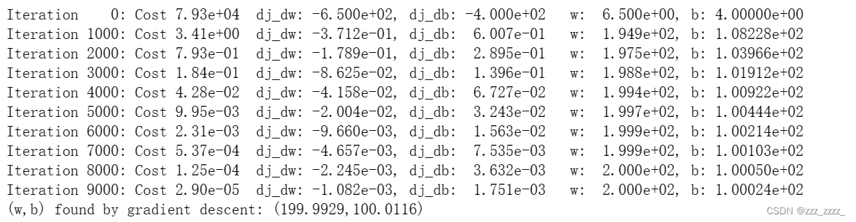 从这个输出中可以看出,随着迭代次数的增加,两个偏导越来越小了,成本也越来越小了
最终求得w为199.9929,b为100.0116
7.成本函数的走向图
# plot cost versus iteration
fig, (ax1, ax2) = plt.subplots(1, 2, constrained_layout=True, figsize=(12,4))
ax1.plot(J_hist[:100])
ax2.plot(1000 + np.arange(len(J_hist[1000:])), J_hist[1000:])
ax1.set_title("Cost vs. iteration(start)");  ax2.set_title("Cost vs. iteration (end)")
ax1.set_ylabel('Cost')            ;  ax2.set_ylabel('Cost')
ax1.set_xlabel('iteration step')  ;  ax2.set_xlabel('iteration step')
plt.show()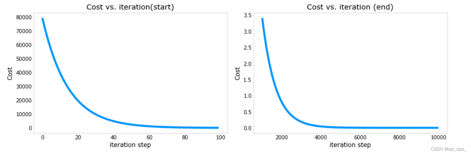
8.预测
print(f"1000 sqft house prediction {w_final*1.0 + b_final:0.1f} Thousand dollars")
print(f"1200 sqft house prediction {w_final*1.2 + b_final:0.1f} Thousand dollars")
print(f"2000 sqft house prediction {w_final*2.0 + b_final:0.1f} Thousand dollars")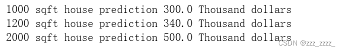
9.学习率过大
# initialize parameters
w_init = 0
b_init = 0
# set alpha to a large value
iterations = 10
tmp_alpha = 8.0e-1
# run gradient descent
w_final, b_final, J_hist, p_hist = gradient_descent(x_train ,y_train, w_init, b_init, tmp_alpha,
                                                    iterations, compute_cost, compute_gradient)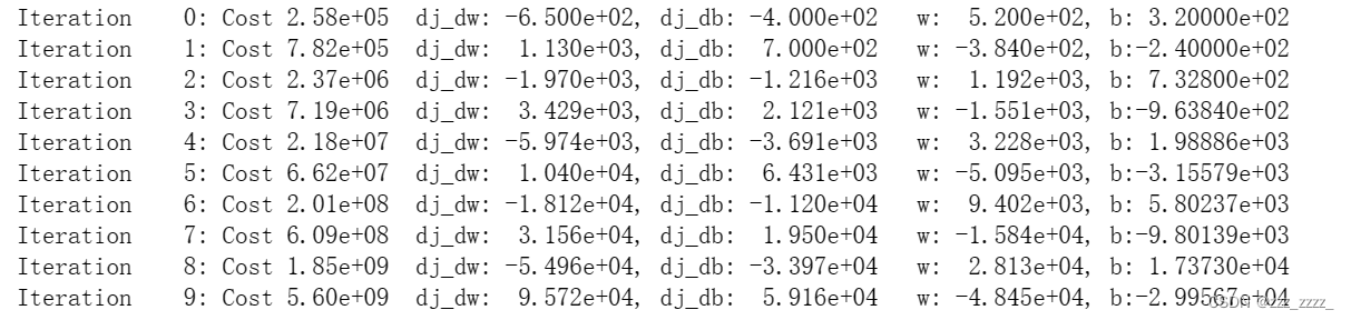
成本越来越大了,就是下图这种情况:


 4395
4395


 被折叠的 条评论
为什么被折叠?
被折叠的 条评论
为什么被折叠?
 到【灌水乐园】发言


