


 本文详细介绍并实现了支持向量机中的SMO(Sequential Minimal Optimization)算法,该算法用于寻找支持向量,即距离分类面最近的数据点。通过具体代码演示了如何在Python中实现这一算法。
(转载请注明出处:http://blog.csdn.net/buptgshengod)
1.背景知识
通过上一节我们通过引入拉格朗日乗子得到支持向量机变形公式。详细变法可以参考这位大神的博客——地址
参照拉格朗日公式F(x1,x2,...λ)=f(x1,x2,...)-λg(x1,x2...)。我们把上面的式子变型为: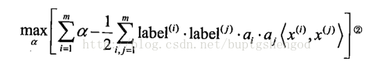
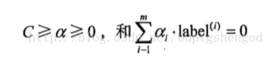
约束条件就变成了:
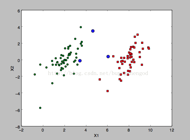
下面就根据最小优化算法SMO(Sequential Minimal Optimization)。找出距离分隔面最近的点,也就是支持向量集。如下图的蓝色点所示。
2.代码
import matplotlib.pyplot as plt
from numpy import *
from time import sleep

def loadDataSet(fileName):
    dataMat = []; labelMat = []
    fr = open(fileName)
    for line in fr.readlines():
        lineArr = line.strip().split('\t')
        dataMat.append([float(lineArr[0]), float(lineArr[1])])
        labelMat.append(float(lineArr[2]))
    return dataMat,labelMat

def selectJrand(i,m):
    j=i #we want to select any J not equal to i
    while (j==i):
        j = int(random.uniform(0,m))
    return j

def clipAlpha(aj,H,L):
    if aj > H:
        aj = H
    if L > aj:
        aj = L
    return aj

def smoSimple(dataMatIn, classLabels, C, toler, maxIter):
    dataMatrix = mat(dataMatIn); labelMat = mat(classLabels).transpose()
    b = 0; m,n = shape(dataMatrix)
    alphas = mat(zeros((m,1)))
    iter = 0
    while (iter < maxIter):
        alphaPairsChanged = 0
        for i in range(m):
            fXi = float(multiply(alphas,labelMat).T*(dataMatrix*dataMatrix[i,:].T)) + b
            Ei = fXi - float(labelMat[i])#if checks if an example violates KKT conditions
            if ((labelMat[i]*Ei < -toler) and (alphas[i] < C)) or ((labelMat[i]*Ei > toler) and (alphas[i] > 0)):
                j = selectJrand(i,m)
                fXj = float(multiply(alphas,labelMat).T*(dataMatrix*dataMatrix[j,:].T)) + b
                Ej = fXj - float(labelMat[j])
                alphaIold = alphas[i].copy(); alphaJold = alphas[j].copy();
                if (labelMat[i] != labelMat[j]):
                    L = max(0, alphas[j] - alphas[i])
                    H = min(C, C + alphas[j] - alphas[i])
                else:
                    L = max(0, alphas[j] + alphas[i] - C)
                    H = min(C, alphas[j] + alphas[i])
#                 if L==H: print "L==H"; continue
                eta = 2.0 * dataMatrix[i,:]*dataMatrix[j,:].T - dataMatrix[i,:]*dataMatrix[i,:].T - dataMatrix[j,:]*dataMatrix[j,:].T
                if eta >= 0: print "eta>=0"; continue
                alphas[j] -= labelMat[j]*(Ei - Ej)/eta
                alphas[j] = clipAlpha(alphas[j],H,L)
#                 if (abs(alphas[j] - alphaJold) < 0.00001): print "j not moving enough"; continue
                alphas[i] += labelMat[j]*labelMat[i]*(alphaJold - alphas[j])#update i by the same amount as j
                                                                        #the update is in the oppostie direction
                b1 = b - Ei- labelMat[i]*(alphas[i]-alphaIold)*dataMatrix[i,:]*dataMatrix[i,:].T - labelMat[j]*(alphas[j]-alphaJold)*dataMatrix[i,:]*dataMatrix[j,:].T
                b2 = b - Ej- labelMat[i]*(alphas[i]-alphaIold)*dataMatrix[i,:]*dataMatrix[j,:].T - labelMat[j]*(alphas[j]-alphaJold)*dataMatrix[j,:]*dataMatrix[j,:].T
                if (0 < alphas[i]) and (C > alphas[i]): b = b1
                elif (0 < alphas[j]) and (C > alphas[j]): b = b2
                else: b = (b1 + b2)/2.0
                alphaPairsChanged += 1
#                 print "iter: %d i:%d, pairs changed %d" % (iter,i,alphaPairsChanged)
        if (alphaPairsChanged == 0): iter += 1
        else: iter = 0
#         print "iteration number: %d" % iter

    return b,alphas

def matplot(dataMat,lableMat):
    xcord1 = []; ycord1 = []
    xcord2 = []; ycord2 = []
    xcord3 = []; ycord3 = []
    for i in range(100):
        if lableMat[i]==1:
           xcord1.append(dataMat[i][0])
           ycord1.append(dataMat[i][1])
        else:
           xcord2.append(dataMat[i][0])
           ycord2.append(dataMat[i][1])
    b,alphas=smoSimple(dataMat,labelMat,0.6,0.001,40)
    for j in range(100):
        if alphas[j]>0:
             xcord3.append(dataMat[j][0])
             ycord3.append(dataMat[j][1])
    fig = plt.figure()
    ax = fig.add_subplot(111)

    ax.scatter(xcord1, ycord1, s=30, c='red', marker='s')
    ax.scatter(xcord2, ycord2, s=30, c='green')
    ax.scatter(xcord3, ycord3, s=80, c='blue')
    ax.plot()
    plt.xlabel('X1'); plt.ylabel('X2');
    plt.show()

if __name__=='__main__':
     dataMat,labelMat=loadDataSet('/Users/hakuri/Desktop/testSet.txt')
#      b,alphas=smoSimple(dataMat,labelMat,0.6,0.001,40)
#      print b,alphas[alphas>0]
     matplot(dataMat,labelMat)


 217
217

 被折叠的 条评论
为什么被折叠?
被折叠的 条评论
为什么被折叠?
 到【灌水乐园】发言


