


- Review of concepts of supervised learning
- boosted trees
- how to define F the space of functions containing all regression trees
- map concept of tree to optimization
- refine the definition of tree
- Define the Complexity of Tree
- revisit the instance set in leaf j as
- The structure score
- EXAMPLE
- search algorithm for single tree
- Efficient Finding of the Best Split
- Algorithm for Split Finding
- What about Categorical Variables
- Pruning and Regularization
- Recap Boosted Tree Algorithm
Review of concepts of supervised learning
objective function
where L(Θ) is the training loss,and Ω(Θ) is regularization which measures the complexity of model.
loss function L(Θ)
- square loss: l(yi,ŷ i)=∥yi−ŷ i∥2
- logistic loss: l(yi,ŷ i)=yiln(1+e−ŷ i)+ŷ iln(1+e−yi)
regularization Ω(Θ)
- l1 norm (lasso): Ω(w)=λ∥w∥1
- l2 norm (ridge): Ω(w)=λ∥w∥22
lasso
- linear model,square loss,l1 regularition
ridge regression
- linear model,square loss,l2 regularition
logistic regression
- linear model, logistic loss,l2 regulation
boosted trees
Regression tree(CART)
regression tree, or classification and regression tree,contains one score in each leaf value.
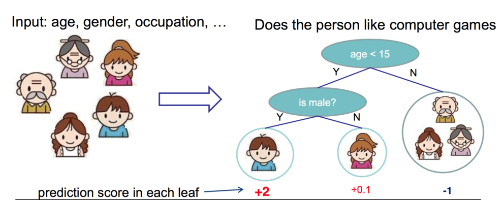
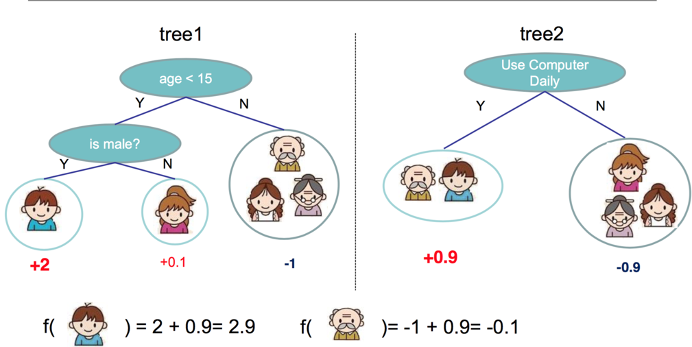
Regression tree ensemble
prediction of each menber is sum of scores predicted by each of the tree
tree ensemble methods
- mostly widely used ,such as GBM,random forest …
- invariante to scaling of inputs,so needn’t worry about feature normalization
- learn higehr order interaction between features
represent the RT in optimization method
model: assuming we have K trees
ŷ i=∑k=1Kfk(xi),fk(x)∈F- F is space of functions containing all regression trees.
- regression tree is a function that maps the attitute to the score.
- each regression tree fk(x) is in charge of some parts of the attributes.
Parametres: struction of each tree fk(x) ,and the score in the leaf
or simply Θ={f1,…,fK}Objective
Obj(Θ)=∑i=1nl(yi,ŷ i)+∑k=1KΩ(fk)(2.3)- how to define to define
Ω
?
- # nodes/depth
- l2 norm of the leaf weights
- ….
- how to define loss function
- square loss result in common gradient boosted machine
- logistic loss result in logitBoost
how to solve the optimization problem
additive training (boosting)
at training round 0,start from constant prediction, add a new function each time:
ŷ (0)i=0
ŷ (1)i=f1(xi)=ŷ (0)i+f1(xi)
ŷ (2)i=f1(xi)+f2(xi)=ŷ (1)i+f2(xi)
…
at traing round t,Keep functions added in previous round(
ŷ (k−1)i
) and add a new function
fk(xi)
:
ŷ (t)i=∑k=1tfk(xi)=ŷ (k−1)i+fk(xi)
how we decide which f to add?
at round t,solve the optimization:
for lose function:
- square loss: Obj(t) becomes a quadratic function of ft , let the derivetive be 0 then…
- other cases ,we can use the numeric ways:
- define gi=∂ŷ (t−1)l(yi,ŷ (t−1)i) , hi=∂2ŷ (t−1)l(yi,ŷ (t−1)i)
- the taylor expansion of
Obj(t)
:
Obj(t)≈∑i=1n[l(yi,ŷ (t−1)i)+gift(xi)+12h2ift(xi)]+Ω(ft)+C - with constants removed,
Obj(t)
becomes:
∑i=1n[gift(xi)+12h2ift(xi)]+Ω(ft)
so again we retain to a quadratic convex optimization.
how to define F: the space of functions containing all regression trees
map concept of tree to optimization
information gain -> train loss
pruning->regularization defined be #nodes
max depth -> constraint on the function space
smoothing leaf values -> l2 regularization on leaf weights
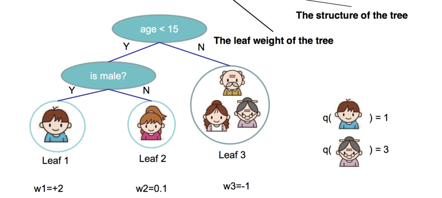
refine the definition of tree
- We define tree by a vector of scores in leafs, and a leaf index mapping function
q(x)
that maps an instance to a leaf
ft(x)=wq(x),w∈RT,q:Rd→{1,2,…,T}
- T is # leaf
- q(x) means that sample falls into which leaf,such as 1,3
- wy means the weight of leaf y
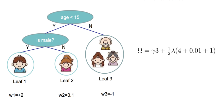
Define the Complexity of Tree
- Define complexity as (this is not the only possible definition)
Ω(ft)=γT+12λ∑j=1Tw2j
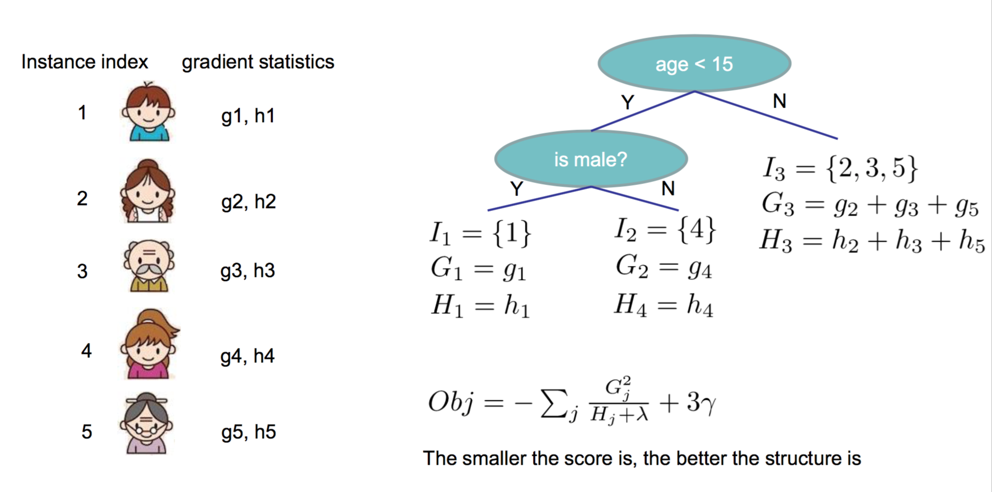
revisit the instance set in leaf j as
- Define the instance set in leaf j as
Ij={i|q(xi)=j} - Regroup the objective by each leaf
Obj(t)≈∑i=1n[gift(xi)+12h2ift(xi)]+Ω(ft)=∑i=1n[gift(xi)+12h2ift(xi)]+γT+12λ∑j=1Tw2j=∑j=1T[∑i∈Ijgiwj+12(∑i∈Ijhi+λ)w2j]+γT
• This is sum of T independent quadratic functions
The structure score
Two facts about single variable quadratic function:
define Gj=∑i∈Ijgj,Hj=∑i∈Ijhj ,then objective becomes
- Assume the structure of tree
q(x)
is fixed, the optimal weight in each leaf, and the resulting objective value are:
w∗j=−GjHj+λ - then objective becomes:
Obj=−12∑j=1TG2jHj+λ+γT
EXAMPLE
here comes the example
search algorithm for single tree
- enumerate the possible tree structures q(x)
- Calculate the according structure score for the q(x), using the scoring function:
Obj=−12∑j=1TG2jHj+λ+γT - find the best tree structure,and use the optimal leaf weight
w∗j=−G2jHj+λ
But… there can be infinite possible tree structures..
so in practice we do not enumerate but greedly grow the tree:
- start from tree with depth 0
For each leaf node of the tree, try to add a split. The change of
objective after adding the split is:
Gain=G2LHL+λ+G2RHR+λ−(GL+GR)2HL+HR+λ−γ- the score of left/right child : G2LHL+λ & G2RHR+λ
- the score of if we do not split : (GL+GR)2HL+HR+λ
- The complexity cost by introducing additional leaf: γ
Remaining question: how do we find the best split?
Efficient Finding of the Best Split
first take a look at the Algorithm for Split Finding
Algorithm for Split Finding
- For each node, enumerate over all features
- For each feature, sorted the instances by feature value
- Use a linear scan to decide the best split along that feature
- Take the best split solution along all the features
Time Complexity growing a tree of depth K is
O(ndKlogn)
,or, each level need
O(nlogn)
time to sort.
There are d features, and we need to do it for K level
- This can be further optimized (e.g. use approximation or caching the sorted features)
- Can scale to very large dataset
Let f and g be two functions defined on some subset of the real numbers. One writes
What about Categorical Variables?
- Some tree learning algorithm handles categorical variable and continuous variable separately.Actually it is not necessary,
- We can easily use the scoring formula we derived to score split based on categorical variables.We can encode the categorical variables into numerical vector
using one-hot encoding. Allocate a #categorical length vector
zj={1,0,if x is in category jothers - The vector will be sparse if there are lots of categories, the learning algorithm is preferred to handle sparse data
Pruning and Regularization
Pre-stopping
- Stop split if the best split have negative gain
- But maybe a split can benefit future splits..
Post-Prunning
- Grow a tree to maximum depth,
- recursively prune all the leaf splits with negative gain
Recap: Boosted Tree Algorithm
- Add a new tree in each iteration
- Beginning of each iteration, calculate gi,hi
- Use the statistics to greedily grow a tree
ft(x)
Obj=−12∑j=1TG2jHj+λ+γT - Add 
ft(x)
to the model
ŷ (t)i=ŷ (t−1)i+ft(xi)
Usually, instead we do ŷ (t)i=ŷ (t−1)i+ϵft(xi)
ϵ is called step-size or shrinkage, usually set around 0.1
This means we do not do full optimization in each step and reserve chance for future rounds, it helps prevent overfitting
Questions 1
How can we build a boosted tree classifier to do weighted regression problem, such that each instance have a importance weight?
- Define objective, calculate, feed it to the old tree learning algorithm we have for un-weighted version
- Again think of separation of model and objective, how does the theory can help better organizing the machine learning toolkit
Questions 2
Back to the time series problem, if I want to learn step functions over time. Is there other ways to learn the time splits, other than the top down split approach?
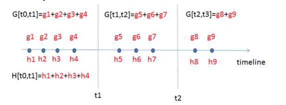
- All that is important is the structure score of the splits
Obj=−12∑j=1TG2jHj+λ+γT
- Top-down greedy, same as trees
- Bottom-up greedy, start from individual points as each group, greedily merge neighbors
- Dynamic programming, can find optimal solution for this case
Summary
• The separation between model, objective, parameters can be helpful for us to understand and customize learning models
• The bias-variance trade-off applies everywhere, including learning in functional space
• We can be formal about what we learn and how we learn. Clear understanding of theory can be used to guide cleaner implementation.


 690
690

 被折叠的 条评论
为什么被折叠?
被折叠的 条评论
为什么被折叠?
 到【灌水乐园】发言


