R语言一元线性回归

最新推荐文章于 2022-12-23 17:24:50 发布

lijinxiu123

最新推荐文章于 2022-12-23 17:24:50 发布

阅读量1.1k

点赞数 1

分类专栏： R语言一元线性回归文章标签： r语言一元线性回归

R语言一元线性回归专栏收录该内容

1 篇文章 0 订阅

订阅专栏

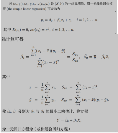
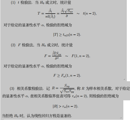
常用三种检验方法

X<-matrix(c(
194.5, 20.79, 1.3179, 131.79,
194.3, 20.79, 1.3179, 131.79,
197.9, 22.40, 1.3502, 135.02,
198.4, 22.67, 1.3555, 135.55,
199.4, 23.15, 1.3646, 136.46,
199.9, 23.35, 1.3683, 136.83,
200.9, 23.89, 1.3782, 137.82,
201.1, 23.99, 1.3800, 138.00,
201.4, 24.02, 1.3806, 138.06,
201.3, 24.01, 1.3805, 138.05,
203.6, 25.14, 1.4004, 140.04,
204.6, 26.57, 1.4244, 142.44,
209.5, 28.49, 1.4547, 145.47,
208.6, 27.76, 1.4434, 144.34,
210.7, 29.04, 1.4630, 146.30,
211.9, 29.88, 1.4754, 147.54,
212.2, 30.06, 1.4780, 147.80),
ncol=4, byrow=T,
dimnames = list(1:17, c("F", "h", "log", "log100")))
forbes<-as.data.frame(X)
plot(forbes$F, forbes$log100)
lm.sol<-lm(log100 ~ F, data=forbes)
summary(lm.sol)

Call:
lm(formula = log100 ~ F, data = forbes)

Residuals:
     Min       1Q   Median       3Q      Max 
-0.32261 -0.14530 -0.06750  0.02111  1.35924 

Coefficients:
             Estimate Std. Error t value Pr(>|t|)    
(Intercept) -42.13087    3.33895  -12.62 2.17e-09 ***
F             0.89546    0.01645   54.45  < 2e-16 ***
---
Signif. codes:  0 ‘***’ 0.001 ‘**’ 0.01 ‘*’ 0.05 ‘.’ 0.1 ‘ ’ 1

Residual standard error: 0.3789 on 15 degrees of freedom
Multiple R-squared:  0.995,	Adjusted R-squared:  0.9946 
F-statistic:  2965 on 1 and 15 DF,  p-value: < 2.2e-16

abline(lm.sol) 将得到的直线方程画在散点图上
y.res<-residuals(lm.sol) 计算回归方程的残差
plot( y.res)

new <- data.frame(x = 0.16) 预测x=0.16时Y的值并给出相应的预测区间
lm.pred<-predict(lm.sol, new, interval="prediction", level=0.95)
lm.pred

fit lwr upr
[1,] 49.42639 46.36621 52.48657