Lesson 4 Part 2 Softmax Regression

首先为了防止混淆,我这里用了自已定义的一些变量

i 在样本中遍历,样本数量为m
j 在特征中遍历,特征数量为n
k 在分类中遍历,分类数量为c

In these notes, we describe the Softmax regression model. This model generalizes logistic regression to classification problems where the class label y can take on more than two possible values. This will be useful for such problems as MNIST digit classification, where the goal is to distinguish between 10 different numerical digits. Softmax regression is a supervised learning algorithm, but we will later be using it in conjuction with our deep learning/unsupervised feature learning methods.
Recall that in logistic regression, we had a training set $\{ (x^{(1)}, y^{(1)}), \ldots, (x^{(m)}, y^{(m)}) \}$ of m labeled examples, where the input features are $x^{(i)} \in \Re^{n+1}$. (In this set of notes, we will use the notational convention of letting the feature vectors x be n + 1 dimensional, with $x_0 = 1$ corresponding to the intercept term.) With logistic regression, we were in the binary classification setting, so the labels were $y^{(i)} \in \{0,1\}$. Our hypothesis took the form:

$$\begin{align} h_\theta(x) = \frac{1}{1+\exp(-\theta^Tx)}, \end{align}$$
and the model parameters θ were trained to minimize the cost function

$$\begin{align} J(\theta) = -\frac{1}{m} \left[ \sum_{i=1}^m y^{(i)} \log h_\theta(x^{(i)}) + (1-y^{(i)}) \log (1-h_\theta(x^{(i)})) \right] \end{align}$$

In the softmax regression setting, we are interested in multi-class classification (as opposed to only binary classification), and so the label y can take on $c$ different values, rather than only two. Thus, in our training set $\{ (x^{(1)}, y^{(1)}), \ldots, (x^{(m)}, y^{(m)}) \}$, we now have that $y^{(i)} \in \{1, 2, \ldots, c\}$. (Note that our convention will be to index the classes starting from 1, rather than from 0.) For example, in the MNIST digit recognition task, we would have $c = 10$ different classes.
Given a test input x, we want our hypothesis to estimate the probability that $p(y = k | x)$ for each value of $k = 1, \ldots, c$. I.e., we want to estimate the probability of the class label taking on each of the $c$ different possible values. Thus, our hypothesis will output a k dimensional vector (whose elements sum to 1) giving us our $c$ estimated probabilities. Concretely, our hypothesis $h_θ(x)$ takes the form:

$$\begin{align} h_\theta(x^{(i)}) = \begin{bmatrix} p(y^{(i)} = 1 | x^{(i)}; \theta) \\ p(y^{(i)} = 2 | x^{(i)}; \theta) \\ \vdots \\ p(y^{(i)} = c | x^{(i)}; \theta) \end{bmatrix} = \frac{1}{ \sum_{k=1}^{c}{e^{ \theta_k^T x^{(i)} }} } \begin{bmatrix} e^{ \theta_1^T x^{(i)} } \\ e^{ \theta_2^T x^{(i)} } \\ \vdots \\ e^{ \theta_c^T x^{(i)} } \\ \end{bmatrix} \end{align}$$
Here $\theta_1, \theta_2, \ldots, \theta_c \in \Re^{n+1}$are the parameters of our model. Notice that the term $\frac{1}{ \sum_{k=1}^{c}{e^{ \theta_k^T x^{(i)} }} }$ normalizes the distribution, so that it sums to one.
For convenience, we will also write $θ$ to denote all the parameters of our model. When you implement softmax regression, it is usually convenient to represent $θ$ as a $c-by-(n + 1)$ matrix obtained by stacking up $\theta_1, \theta_2, \ldots, \theta_k$ in rows, so that

$$\theta = \begin{bmatrix} \mbox{---} \theta_1^T \mbox{---} \\ \mbox{---} \theta_2^T \mbox{---} \\ \vdots \\ \mbox{---} \theta_c^T \mbox{---} \\ \end{bmatrix}$$

Cost Function

We now describe the cost function that we’ll use for softmax regression. In the equation below, $1\{\cdot\}$ is the indicator function, so that 1{a true statement} = 1, and 1{a false statement} = 0. For example, 1{2 + 2 = 4} evaluates to 1; whereas 1{1 + 1 = 5} evaluates to 0. Our cost function will be:

$$\begin{align} J(\theta) = - \frac{1}{m} \left[ \sum_{i=1}^{m} \sum_{k=1}^{c} 1\left\{y^{(i)} = k\right\} \log \frac{e^{\theta_k^T x^{(i)}}}{\sum_{l=1}^c e^{ \theta_l^T x^{(i)} }}\right] \end{align}$$
Notice that this generalizes the logistic regression cost function, which could also have been written:

$$\begin{align} J(\theta) &= -\frac{1}{m} \left[ \sum_{i=1}^m (1-y^{(i)}) \log (1-h_\theta(x^{(i)})) + y^{(i)} \log h_\theta(x^{(i)}) \right] \\ &= - \frac{1}{m} \left[ \sum_{i=1}^{m} \sum_{k=0}^{1} 1\left\{y^{(i)} = k\right\} \log p(y^{(i)} = k | x^{(i)} ; \theta) \right] \end{align}$$
The softmax cost function is similar, except that we now sum over the k different possible values of the class label. Note also that in softmax regression, we have that
$p(y^{(i)} = k | x^{(i)} ; \theta) = \frac{e^{\theta_k^T x^{(i)}}}{\sum_{l=1}^c e^{ \theta_l^T x^{(i)}} }$
.
There is no known closed-form way to solve for the minimum of J(θ), and thus as usual we’ll resort to an iterative optimization algorithm such as gradient descent or L-BFGS. Taking derivatives, one can show that the gradient is:

$$\begin{align} \nabla_{\theta_k} J(\theta) = - \frac{1}{m} \sum_{i=1}^{m}{ \left[ x^{(i)} \left( 1\{ y^{(i)} = k\} - p(y^{(i)} = k | x^{(i)}; \theta) \right) \right] } \end{align}$$

Recall the meaning of the “$\nabla_{\theta_j}$” notation. In particular, $\nabla_{\theta_k} J(\theta)$ is itself a vector, so that its j-th element is $\frac{\partial J(\theta)}{\partial \theta_{kj}}$ the partial derivative of J(θ) with respect to the j-th element of $θ_k$.
Armed with this formula for the derivative, one can then plug it into an algorithm such as gradient descent, and have it minimize J(θ). For example, with the standard implementation of gradient descent, on each iteration we would perform the update $\theta_k := \theta_k - \alpha \nabla_{\theta_k} J(\theta)$ (for each $k=1,\ldots,c$).
When implementing softmax regression, we will typically use a modified version of the cost function described above; specifically, one that incorporates weight decay. We describe the motivation and details below.

Properties of softmax regression parameterization

Softmax regression has an unusual property that it has a “redundant” set of parameters. To explain what this means, suppose we take each of our parameter vectors $θ_k$, and subtract some fixed vector $ψ$ from it, so that every $θ_k$ is now replaced with $θ_k − ψ$ (for every $k=1, \ldots, c$). Our hypothesis now estimates the class label probabilities as

$$\begin{align} p(y^{(i)} = k | x^{(i)} ; \theta) &= \frac{e^{(\theta_k-\psi)^T x^{(i)}}}{\sum_{l=1}^c e^{ (\theta_l-\psi)^T x^{(i)}}} \\ &= \frac{e^{\theta_k^T x^{(i)}} e^{-\psi^Tx^{(i)}}}{\sum_{l=1}^c e^{\theta_l^T x^{(i)}} e^{-\psi^Tx^{(i)}}} \\ &= \frac{e^{\theta_k^T x^{(i)}}}{\sum_{l=1}^c e^{ \theta_l^T x^{(i)}}}. \end{align}$$
In other words, subtracting $ψ$ from every $θ_k$ does not affect our hypothesis’ predictions at all! This shows that softmax regression’s parameters are “redundant.” More formally, we say that our softmax model is overparameterized, meaning that for any hypothesis we might fit to the data, there are multiple parameter settings that give rise to exactly the same hypothesis function hθ mapping from inputs x to the predictions.
Further, if the cost function $J(θ)$ is minimized by some setting of the parameters $(\theta_1, \theta_2,\ldots, \theta_c)$, then it is also minimized by $(\theta_1 - \psi, \theta_2 - \psi,\ldots, \theta_c - \psi)$ for any value of $ψ$. Thus, the minimizer of $J(θ)$ is not unique. (Interestingly, $J(θ)$ is still convex, and thus gradient descent will not run into a local optima problems. But the Hessian is singular/non-invertible, which causes a straightforward implementation of Newton’s method to run into numerical problems.)
Notice also that by setting $ψ = θ_1$, one can always replace $θ_1$ with $\theta_1 - \psi = \vec{0}$(the vector of all 0’s), without affecting the hypothesis. Thus, one could “eliminate” the vector of parameters $θ_1$ (or any other $θ_k$, for any single value of $k$), without harming the representational power of our hypothesis. Indeed, rather than optimizing over the $c(n + 1)$ parameters $(\theta_1, \theta_2,\ldots, \theta_c)$(where $\theta_k \in \Re^{n+1}$), one could instead set $\theta_1 = \vec{0}$ and optimize only with respect to the $(c − 1)(n + 1)$ remaining parameters, and this would work fine.
In practice, however, it is often cleaner and simpler to implement the version which keeps all the parameters $(\theta_1, \theta_2,\ldots, \theta_c)$, without arbitrarily setting one of them to zero. But we will make one change to the cost function: Adding weight decay. This will take care of the numerical problems associated with softmax regression’s overparameterized representation.

但是这里我们除了Weight Decay外,还是减去最大值,原因如下

However, when the products $\theta_k^T x^{(i)}$ are large, the exponential function $e^{\theta_k^T x^{(i)}}$ will become very very large and possibly overflow. To prevent overflow, we can simply subtract some large constant value from each of the $\theta_k^T x^{(i)}$ terms before computing the exponential. In practice, for each example, you can use the maximum of the $\theta_k^T x^{(i)}$terms as the constant.

$$\begin{align} h_\theta(x^{(i)}) &= \frac{1}{ \sum_{k=1}^{c}{e^{ \theta_k^T x^{(i)} }} } \begin{bmatrix} e^{ \theta_1^T x^{(i)} } \\ e^{ \theta_2^T x^{(i)} } \\ \vdots \\ e^{ \theta_c^T x^{(i)} } \\ \end{bmatrix}\\ &= \frac{e^{-a}}{ e^{-a}\sum_{k=1}^{c}{e^{ \theta_k^T x^{(i)} }} } \begin{bmatrix} e^{ \theta_1^T x^{(i)} } \\ e^{ \theta_2^T x^{(i)} } \\ \vdots \\ e^{ \theta_c^T x^{(i)} } \\ \end{bmatrix}\\ &= \frac{1}{ \sum_{k=1}^{c}{e^{ \theta_k^T x^{(i)} -a}} } \begin{bmatrix} e^{ \theta_1^T x^{(i)} -a} \\ e^{ \theta_2^T x^{(i)} -a} \\ \vdots \\ e^{ \theta_c^T x^{(i)} -a} \\ \end{bmatrix}\\ \end{align}$$

这里的a为行向量,其中每列的元素为矩阵$\theta^Tx$对应列$\theta^Tx^{(i)}$中的最大的元素

注意这里$\theta$为$c*n$的矩阵,$x$为$n*m$的矩阵,$\theta^Tx$为$c*m$的矩阵

Weight Decay

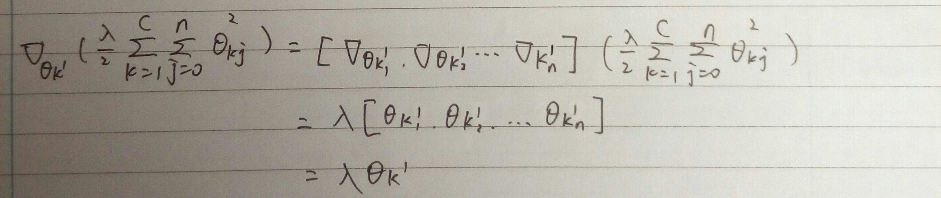
We will modify the cost function by adding a weight decay term $\textstyle \frac{\lambda}{2} \sum_{k=1}^c \sum_{j=0}^{n} \theta_{kj}^2$ which penalizes large values of the parameters. Our cost function is now

$$\begin{align} J(\theta) = - \frac{1}{m} \left[ \sum_{i=1}^{m} \sum_{k=1}^{c} 1\left\{y^{(i)} = k\right\} \log \frac{e^{\theta_k^T x^{(i)}}}{\sum_{l=1}^c e^{ \theta_l^T x^{(i)} }} \right] + \frac{\lambda}{2} \sum_{k=1}^c \sum_{j=0}^n \theta_{kj}^2 \end{align}$$
With this weight decay term (for any $λ > 0$), the cost function $J(θ)$ is now strictly convex, and is guaranteed to have a unique solution. The Hessian is now invertible, and because $J(θ)$ is convex, algorithms such as gradient descent, L-BFGS, etc. are guaranteed to converge to the global minimum.
To apply an optimization algorithm, we also need the derivative of this new definition of $J(θ)$. One can show that the derivative is:
$$\begin{align} \nabla_{\theta_k} J(\theta) = - \frac{1}{m} \sum_{i=1}^{m}{ \left[ x^{(i)} ( 1\{ y^{(i)} = k\} - p(y^{(i)} = k | x^{(i)}; \theta) ) \right] } + \lambda \theta_k \end{align}$$

这里对$J(θ)$求导得到的结果,推导如下：

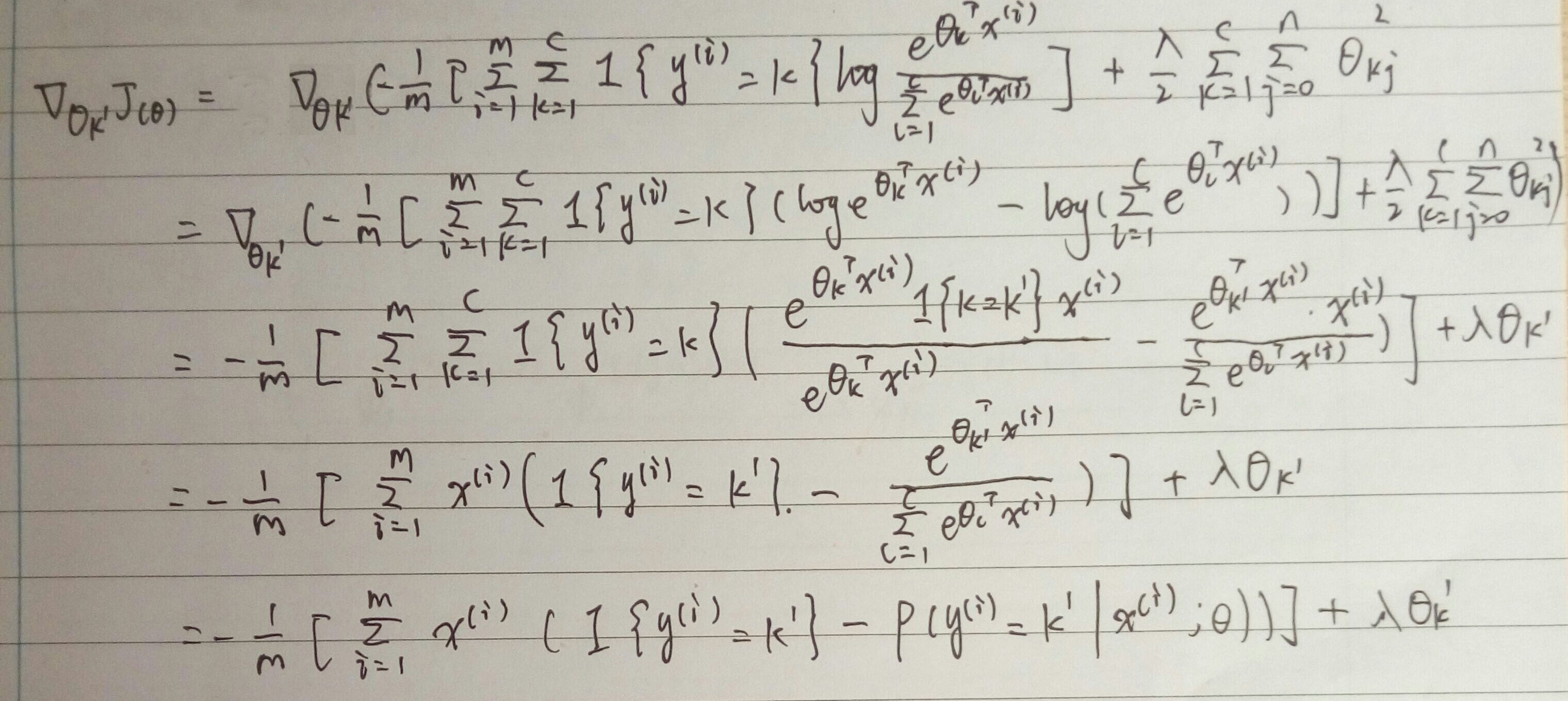
注意这里用到了公式：
$\frac{\partial x^Ta}{\partial x} = \frac{\partial a^Tx}{\partial x} = a$ (引用于matrix cookbook 2.4.1)

note: In particular, $\nabla_{\theta_k} J(\theta)$ is itself a vector, so that its j-th element is $\frac{\partial J(\theta)}{\partial \theta_{kj}}$ the partial derivative of J(θ) with respect to the j-th element of $θ_k$.

By minimizing $J(θ)$ with respect to θ <script type="math/tex" id="MathJax-Element-87">θ</script>, we will have a working implementation of softmax regression.

下面提供源码

// Softmax regression

#include <iostream>
#include <armadillo>
#include <math.h>
using namespace arma;
using namespace std;

#define elif else if
#define MAX_ITER 1000000

double cost = 0.0;
mat grad;
double lrate = 0.1;
double lambda = 0.0;
int nclasses = 2;

colvec vec2colvec(vector<double>& vec) {
    int length = vec.size();
    colvec A(length);
    for (int i = 0; i<length; i++) {
        A(i) = vec[i];
    }
    return A;
}

rowvec vec2rowvec(vector<double>& vec) {
    colvec A = vec2colvec(vec);
    return A.t();
}

mat vec2mat(vector<vector<double> >&vec) {
    int cols = vec.size();
    int rows = vec[0].size();
    mat A(rows, cols);
    for (int i = 0; i<rows; i++) {
        for (int j = 0; j<cols; j++) {
            A(i, j) = vec[j][i];
        }
    }
    return A;
}

void update_CostFunction_and_Gradient(mat x, rowvec y, mat weightsMatrix, double lambda) {

    int nsamples = x.n_cols;
    int nfeatures = x.n_rows;
    //calculate cost function
    mat theta(weightsMatrix);
    mat M = theta * x;
    mat temp = repmat(max(M, 0), nclasses, 1);
    M = M - temp;
    M = arma::exp(M);
    temp = repmat(sum(M, 0), nclasses, 1);
    M = M / temp;

    mat groundTruth = zeros<mat>(nclasses, nsamples);
    for (int i = 0; i<y.size(); i++) {
        groundTruth(y(i), i) = 1;//对y的数据进行归类
    }
    temp = groundTruth % (arma::log(M));
    cost = -accu(temp) / nsamples;
    cost += accu(arma::pow(theta, 2)) * lambda / 2;

    //calculate gradient
    temp = groundTruth - M;
    temp = temp * x.t();
    grad = -temp / nsamples;
    grad += lambda * theta;
}

rowvec calculateY(mat x, mat weightsMatrix) {

    mat theta(weightsMatrix);
    mat M = theta * x;
    mat temp = repmat(max(M, 0), nclasses, 1);
    M = M - temp;
    M = arma::exp(M);
    temp = repmat(sum(M, 0), nclasses, 1);
    M = M / temp;
    M = arma::log(M);
    rowvec result = zeros<rowvec>(M.n_cols);
    for (int i = 0; i<M.n_cols; i++) {
        int maxele = INT_MIN;
        int which = 0;
        for (int j = 0; j<M.n_rows; j++) {
            if (M(j, i) > maxele) {
                maxele = M(j, i);
                which = j;
            }
        }
        result(i) = which;
    }
    return result;
}

void softmax(vector<vector<double> >&vecX, vector<double> &vecY, vector<vector<double> >& testX, vector<double>& testY) {

    int nsamples = vecX.size();
    int nfeatures = vecX[0].size();
    //change vecX and vecY into matrix or vector.
    rowvec y = vec2rowvec(vecY);
    mat x = vec2mat(vecX);

    double init_epsilon = 0.12;
    mat weightsMatrix = randu<mat>(nclasses, nfeatures);
    weightsMatrix = weightsMatrix * (2 * init_epsilon) - init_epsilon;
    grad = zeros<mat>(nclasses, nfeatures);

    /*
    //Gradient Checking (remember to disable this part after you're sure the
    //cost function and dJ function are correct)
    update_CostFunction_and_Gradient(x, y, weightsMatrix, lambda);
    mat dJ(grad);
    cout<<"test!!!!"<<endl;
    double epsilon = 1e-4;
    for(int i=0; i<weightsMatrix.n_rows; i++){
    for(int j=0; j<weightsMatrix.n_cols; j++){
    double memo = weightsMatrix(i, j);
    weightsMatrix(i, j) = memo + epsilon;
    update_CostFunction_and_Gradient(x, y, weightsMatrix, lambda);
    double value1 = cost;
    weightsMatrix(i, j) = memo - epsilon;
    update_CostFunction_and_Gradient(x, y, weightsMatrix, lambda);
    double value2 = cost;
    double tp = (value1 - value2) / (2 * epsilon);
    cout<<i<<", "<<j<<", "<<tp<<", "<<dJ(i, j)<<endl;
    weightsMatrix(i, j) = memo;
    }
    }
    */

    int converge = 0;
    double lastcost = 0.0;
    while (converge < MAX_ITER) {
        update_CostFunction_and_Gradient(x, y, weightsMatrix, lambda);
        weightsMatrix -= lrate * grad;

        cout << "learning step: " << converge << ", Cost function value = " << cost << endl;
        if (fabs((cost - lastcost)) <= 5e-6 && converge > 0) break;
        lastcost = cost;
        ++converge;
    }
    cout << "############result#############" << endl;

    rowvec yT = vec2rowvec(testY);
    mat xT = vec2mat(testX);
    rowvec result = calculateY(xT, weightsMatrix);
    rowvec error = yT - result;
    int correct = error.size();
    for (int i = 0; i<error.size(); i++) {
        if (error(i) != 0) --correct;
    }
    cout << "correct: " << correct << ", total: " << error.size() << ", accuracy: " << double(correct) / (double)(error.size()) << endl;

}

int main(int argc, char** argv)
{
    long start, end;
    //read training X from .txt file
    FILE *streamX, *streamY;
    streamX = fopen("trainX.txt", "r");
    int numofX = 30;
    vector<vector<double> > vecX;
    double tpdouble;
    int counter = 0;
    while (1) {
        if (fscanf(streamX, "%lf", &tpdouble) == EOF) break;
        if (counter / numofX >= vecX.size()) {
            vector<double> tpvec;
            vecX.push_back(tpvec);
        }
        vecX[counter / numofX].push_back(tpdouble);
        ++counter;
    }
    fclose(streamX);

    cout << vecX.size() << ", " << vecX[0].size() << endl;

    //read training Y from .txt file
    streamY = fopen("trainY.txt", "r");
    vector<double> vecY;
    while (1) {
        if (fscanf(streamY, "%lf", &tpdouble) == EOF) break;
        vecY.push_back(tpdouble);
    }
    fclose(streamY);

    for (int i = 1; i<vecX.size(); i++) {
        if (vecX[i].size() != vecX[i - 1].size()) return 0;
    }
    if (vecX.size() != vecY.size()) return 0;

    streamX = fopen("testX.txt", "r");
    vector<vector<double> > vecTX;
    counter = 0;
    while (1) {
        if (fscanf(streamX, "%lf", &tpdouble) == EOF) break;
        if (counter / numofX >= vecTX.size()) {
            vector<double> tpvec;
            vecTX.push_back(tpvec);
        }
        vecTX[counter / numofX].push_back(tpdouble);
        ++counter;
    }
    fclose(streamX);

    streamY = fopen("testY.txt", "r");
    vector<double> vecTY;
    while (1) {
        if (fscanf(streamY, "%lf", &tpdouble) == EOF) break;
        vecTY.push_back(tpdouble);
    }
    fclose(streamY);

    start = clock();
    softmax(vecX, vecY, vecTX, vecTY);
    end = clock();
    cout << "Training used time: " << ((double)(end - start)) / CLOCKS_PER_SEC << " second" << endl;
    return 0;
}

然后,对照源码我们看下该算法是如何实现的

FILE *streamX, *streamY;
    streamX = fopen("trainX.txt", "r");
    int numofX = 30;
    vector<vector<double> > vecX;
    double tpdouble;
    int counter = 0;
    while (1) {
        if (fscanf(streamX, "%lf", &tpdouble) == EOF) break;
        if (counter / numofX >= vecX.size()) {
            vector<double> tpvec;
            vecX.push_back(tpvec);
        }
        vecX[counter / numofX].push_back(tpdouble);
        ++counter;
    }
    fclose(streamX);

这部分将trainX.txt的数据读入vecX中,
trainX.txt每行有30个数据,一共有284行
所以vecX外层大小为284, 内层大小为30
表示成矩阵 284 * 30

同理,我们来看TrainY.txt的数据

    //read training Y from .txt file
    streamY = fopen("trainY.txt", "r");
    vector<double> vecY;
    while (1) {
        if (fscanf(streamY, "%lf", &tpdouble) == EOF) break;
        vecY.push_back(tpdouble);
    }
    fclose(streamY);

trainY.txt每行有1个数据,一共有284行
表示成矩阵 284 * 1

同理, testX 和 textY 分别跟 trainX 和 trainY一样大小

然后我们看softmax函数

    int nsamples = vecX.size();//284
    int nfeatures = vecX[0].size();//30
    //change vecX and vecY into matrix or vector.
    rowvec y = vec2rowvec(vecY);
    mat x = vec2mat(vecX);// x 30 * 284

    double init_epsilon = 0.12;
    mat weightsMatrix = randu<mat>(nclasses, nfeatures);//weightsMatrix 2 * 30 这个矩阵就是需要求的θ系数.对于每种分类,对应一个不同的θ向量,该向量有n个分量
    weightsMatrix = weightsMatrix * (2 * init_epsilon) - init_epsilon;//给需要求的θ一个初值
    grad = zeros<mat>(nclasses, nfeatures); //grad 2 * 30

    int converge = 0;
    double lastcost = 0.0;
    while (converge < MAX_ITER) {
        update_CostFunction_and_Gradient(x, y, weightsMatrix, lambda);
        weightsMatrix -= lrate * grad;

        cout << "learning step: " << converge << ", Cost function value = " << cost << endl;
        if (fabs((cost - lastcost)) <= 5e-6 && converge > 0) break;
        lastcost = cost;
        ++converge;

接着我们看下update_CostFunction_and_Gradient

void update_CostFunction_and_Gradient(mat x, rowvec y, mat weightsMatrix, double lambda) {

    int nsamples = x.n_cols;//284
    int nfeatures = x.n_rows;//30
    //calculate cost function
    mat theta(weightsMatrix);
    mat M = theta * x; // theta:2*30   x:30*284   M:2*284
    mat temp = repmat(max(M, 0), nclasses, 1); // temp:2*284  每列中元素相同,为M对应列中的最大的元素
    M = M - temp;//相当于上面描述中减去a
    M = arma::exp(M);//分子
    temp = repmat(sum(M, 0), nclasses, 1);//分母
    M = M / temp;

    mat groundTruth = zeros<mat>(nclasses, nsamples);//groundTruth: 2*284
    for (int i = 0; i<y.size(); i++) { // y:284*1
        groundTruth(y(i), i) = 1;//对y的数据进行归类
    }
    temp = groundTruth % (arma::log(M));//grounTruth相当1{y(i)=k}
    cost = -accu(temp) / nsamples;
    cost += accu(arma::pow(theta, 2)) * lambda / 2;

    //calculate gradient
    temp = groundTruth - M;
    temp = temp * x.t();
    grad = -temp / nsamples;
    grad += lambda * theta;
}

然后后面就是用梯度下降法进行迭代，代码我就不多解释了

源代及数据参照这里

由于源代码应用到armadillo,关于armadillo的安装请参照这里