Histogram of Oriented Gradients and Object Detection

Histogram of Oriented Gradients and Object Detection

http://www.pyimagesearch.com/2014/11/10/histogram-oriented-gradients-object-detection/

by  Adrian Rosebrock  on  November 10, 2014  in  Machine Learning, Tutorials

If you’ve been paying attention to my Twitter account lately, you’ve probably noticed one or twoteasers of what I’ve been working on — a Python framework/package to rapidly construct object detectors using Histogram of Oriented Gradients and Linear Support Vector Machines.

Honestly, I really can’t stand using the Haar cascade classifiers provided by OpenCV (i.e. the Viola-Jones detectors) — and hence why I’m working on my own suite of classifiers. While cascade methods are extremely fast, they leave much to be desired. If you’ve ever used OpenCV to detect faces you’ll know exactly what I’m talking about.

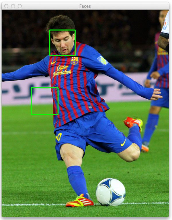
Figure 1: Example of falsely detecting a face in an image. This is a common problem when using cv2.detectMultiScale.

In order to detect faces/humans/objects/whatever in OpenCV (and remove the false positives), you’ll spend a lot of time tuning the  cv2.detectMultiScale  parameters. And again, there is no guarantee that the exact same parameters will work from image-to-image. This makes batch-processing large datasets for face detection a tedious task since you’ll be very concerned with either (1) falsely detecting faces or (2) missing faces entirely, simply due to poor parameter choices on a per image basis.

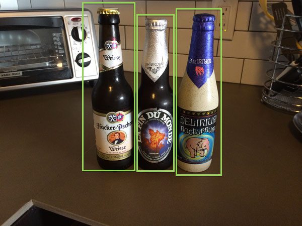
There is also the problem that the Viola-Jones detectors are nearing 15 years old. If this detector were a nice bottle of Cabernet Sauvignon I might be pretty stoked right now. But the field has advanced substantially since then.  Back in 2001 the Viola-Jones detectors were state-of-the-art and they were certainly a huge motivating force behind the incredible new advances we have in object detection today.

Now, the Viola-Jones detector isn’t our only choice for object detection. We have object detection using keypoints, local invariant descriptors, and bag-of-visual-words models. We have Histogram of Oriented Gradients. We have deformable parts models. Exemplar models. And we are now utilizing Deep Learning with pyramids to recognize objects at different scales!

All that said, even though the Histogram of Oriented Gradients descriptor for object recognition is nearly a decade old, it is still heavily used today — and with fantastic results. The Histogram of Oriented Gradients method suggested by Dalal and Triggs in their seminal 2005 paper, Histogram of Oriented Gradients for Human Detection demonstrated that the Histogram of Oriented Gradients (HOG) image descriptor and a Linear Support Vector Machine (SVM) could be used to train highly accurate object classifiers — or in their particular study, human detectors.

Histogram of Oriented Gradients and Object Detection

I’m not going to review the entire detailed process of training an object detector using Histogram of Oriented Gradients (yet), simply because each step can be fairly detailed. But I wanted to take a minute and detail the general algorithm for training an object detector using Histogram of Oriented Gradients. It goes a little something like this:

Step 1:

Sample P positive samples from your training data of the object(s) you want to detect and extract HOG descriptors from these samples.

Step 2:

Sample N negative samples from a negative training set that does not contain any of the objects you want to detect and extract HOG descriptors from these samples as well. In practice N >> P.

Step 3:

Train a Linear Support Vector Machine on your positive and negative samples.

Step 4:

Figure 2: Example of the sliding a window approach, where we slide a window from left-to-right and top-to-bottom. Note: Only a single scale is sown. In practice this window would be applied to multiple scales of the image.

Apply hard-negative mining. For each image and each possible scale of each image in your negative training set, apply the sliding window technique and slide your window across the image. At each window compute your HOG descriptors and apply your classifier. If your classifier (incorrectly) classifies a given window as an object (and it will, there will absolutely be false-positives), record the feature vector associated with the false-positive patch along with the probability of the classification. This approach is called hard-negative mining.

Step 5:

Take the false-positive samples found during the hard-negative mining stage, sort them by their confidence (i.e. probability) and re-train your classifier using these hard-negative samples. (Note: You can iteratively apply steps 4-5, but in practice one stage of hard-negative mining usually [not not always] tends to be enough. The gains in accuracy on subsequent runs of hard-negative mining tend to be minimal.)

Step 6:

Your classifier is now trained and can be applied to your test dataset. Again, just like in Step 4, for each image in your test set, and for each scale of the image, apply the sliding window technique. At each window extract HOG descriptors and apply your classifier. If your classifier detects an object with sufficiently large probability, record the bounding box of the window. After you have finished scanning the image, apply non-maximum suppression to remove redundant and overlapping bounding boxes.

These are the bare minimum steps required, but by using this 6-step process you can train and build object detection classifiers of your own! Extensions to this approach include a deformable parts model and Exemplar SVMs, where you train a classifier for each positive instance rather than a collection of them.

However, if you’ve ever worked with object detection in images you’ve likely ran into the problem of detecting multiple bounding boxes around the object you want to detect in the image.

Here’s an example of this overlapping bounding box problem:

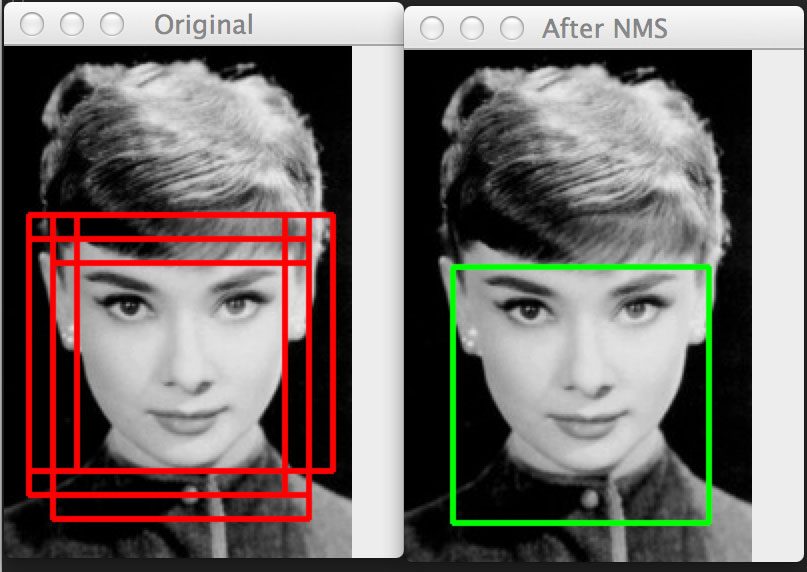
Figure 3: (Left) Detecting multiple overlapping bounding boxes around the face we want to detect. (Right) Applying non-maximum suppression to remove the redundant bounding boxes.

Notice on the left we have 6 overlapping bounding boxes that have correctly detected Audrey Hepburn’s face. However, these 6 bounding boxes all refer to the same face — we need a method to suppress the 5 smallest bounding boxes in the region, keeping only the largest one, as seen on the right.

This is a common problem, no matter if you are using the Viola-Jones based method or following the Dalal-Triggs paper.

There are multiple ways to remedy this problem. Triggs et al. suggests to use the Mean-Shift algorithm to detect multiple modes in the bounding box space by utilizing the (x, y) coordinates of the bounding box as well as the logarithm of the current scale of the image.

I’ve personally tried this method and wasn’t satisfied with the results. Instead, you’re much better off relying on a strong classifier with higher accuracy (meaning there are very few false positives) and then applying non-maximum suppression to the bounding boxes.

I spent some time looking for a good non-maximum suppression (sometimes called non-maxima suppression) implementation in Python. When I couldn’t find one, I chatted with my friend Dr. Tomasz Malisiewicz, who has spent his entire career working with object detector algorithms and the HOG descriptor. There is literally no one that I know who has more experience in this area than Tomasz. And if you’ve ever read any of his papers, you’ll know why. His work is fantastic.

Anyway, after chatting with him, he pointed me to two MATLAB implementations. The first is based on the work by Felzenszwalb et al. and their deformable parts model.

The second method is implemented by Tomasz himself for his Exemplar SVM project which he used for his dissertation and his ICCV 2011 paper, Ensemble of Exemplar-SVMs for Object Detection and Beyond. It’s important to note that Tomasz’s method is over 100x faster than the Felzenszwalb et al. method. And when you’re executing your non-maximum suppression function millions of times, that 100x speedup really matters.

I’ve implemented both the Felzenszwalb et al. and Tomasz et al. methods, porting them from MATLAB to Python. Next week we’ll start with the Felzenszwalb method, then the following week I’ll cover Tomasz’s method. While Tomasz’s method is substantially faster, I think it’s important to see both implementations so we can understand exactly why his method obtains such drastic speedups.

Be sure to stick around and check out these posts! These are absolutely critical steps to building object detectors of your own!

Summary

In this blog post we had a little bit of a history lesson regarding object detectors. We also had a sneak peek into a Python framework that I am working on for object detection in images.

From there we had a quick review of how the Histogram of Oriented Gradients method is used in conjunction with a Linear SVM to train a robust object detector.

However, no matter what method of object detection you use, you will likely end up with multiple bounding boxes surrounding the object you want to detect. In order to remove these redundant boxes you’ll need to apply Non-Maximum Suppression.

Over the next two weeks I’ll show you two implementations of Non-Maximum Suppression that you can use in your own object detection projects.

Be sure to enter your email address in the form below to receive an announcement when these posts go live! Non-Maximum Suppression is absolutely critical to obtaining an accurate and robust object detection system using HOG, so you definitely don’t want to miss these posts!