Deep learning------------PCA (principle component analysis)

最新推荐文章于 2022-06-06 23:39:24 发布

jingruixiaozhuang

最新推荐文章于 2022-06-06 23:39:24 发布

阅读量1.2k

点赞数

分类专栏： Deep Learning

本文链接：https://blog.csdn.net/u012796064/article/details/17147711

版权

Deep Learning 专栏收录该内容

26 篇文章 2 订阅

订阅专栏

PCA在 stanford CS229课程里有详细的讲解：

一下是对PCA从各个方面的深入剖析：

Introduction

Principal Components Analysis (PCA) is a dimensionality reduction algorithm that can be used to significantly speed up your unsupervised feature learning algorithm. More importantly, understanding PCA will enable us to later implement whitening, which is an important pre-processing step for many algorithms.

Suppose you are training your algorithm on images. Then the input will be somewhat redundant, because the values of adjacent pixels in an image are highly correlated. Concretely, suppose we are training on 16x16 grayscale image patches. Then $\textstyle x \in \Re^{256}$ are 256 dimensional vectors, with one feature $\textstyle x_j$ corresponding to the intensity of each pixel. Because of the correlation between adjacent pixels, PCA will allow us to approximate the input with a much lower dimensional one, while incurring very little error.

Example and Mathematical Background

For our running example, we will use a dataset 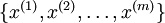$\textstyle \{x^{(1)}, x^{(2)}, \ldots, x^{(m)}\}$ with $\textstyle n=2$ dimensional inputs, so that $\textstyle x^{(i)} \in \Re^2$ . Suppose we want to reduce the data from 2 dimensions to 1. (In practice, we might want to reduce data from 256 to 50 dimensions, say; but using lower dimensional data in our example allows us to visualize the algorithms better.) Here is our dataset:

This data has already been pre-processed so that each of the features $\textstyle x_1$ and $\textstyle x_2$ have about the same mean (zero) and variance.

For the purpose of illustration, we have also colored each of the points one of three colors, depending on their $\textstyle x_1$ value; these colors are not used by the algorithm, and are for illustration only.

PCA will find a lower-dimensional subspace onto which to project our data. From visually examining the data, it appears that $\textstyle u_1$ is the principal direction of variation of the data, and $\textstyle u_2$ the secondary direction of variation:

I.e., the data varies much more in the direction $\textstyle u_1$ than $\textstyle u_2$ . To more formally find the directions $\textstyle u_1$ and $\textstyle u_2$ , we first compute the matrix $\textstyle \Sigma$ as follows:

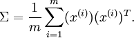
$\begin{align}\Sigma = \frac{1}{m} \sum_{i=1}^m (x^{(i)})(x^{(i)})^T. \end{align}$

If $\textstyle x$ has zero mean, then $\textstyle \Sigma$ is exactly the covariance matrix of $\textstyle x$ . (The symbol " $\textstyle \Sigma$ ", pronounced "Sigma", is the standard notation for denoting the covariance matrix. Unfortunately it looks just like the summation symbol, as in $\sum_{i=1}^n i$ ; but these are two different things.)

It can then be shown that $\textstyle u_1$ ---the principal direction of variation of the data---is the top (principal) eigenvector of $\textstyle \Sigma$ , and $\textstyle u_2$ is the second eigenvector.

Note: If you are interested in seeing a more formal mathematical derivation/justification of this result, see the CS229 (Machine Learning) lecture notes on PCA (link at bottom of this page). You won't need to do so to follow along this course, however.

You can use standard numerical linear algebra software to find these eigenvectors (see Implementation Notes). Concretely, let us compute the eigenvectors of $\textstyle \Sigma$ , and stack the eigenvectors in columns to form the matrix $\textstyle U$ :

$\begin{align}U = \begin{bmatrix} | & | & & | \\u_1 & u_2 & \cdots & u_n \\| & | & & | \end{bmatrix} \end{align}$

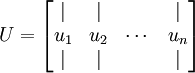
Here, $\textstyle u_1$ is the principal eigenvector (corresponding to the largest eigenvalue), $\textstyle u_2$ is the second eigenvector, and so on. Also, let 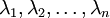$\textstyle \lambda_1, \lambda_2, \ldots, \lambda_n$ be the corresponding eigenvalues.

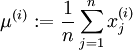
The vectors $\textstyle u_1$ and $\textstyle u_2$ in our example form a new basis in which we can represent the data. Concretely, let $\textstyle x \in \Re^2$ be some training example. Then $\textstyle u_1^Tx$ is the length (magnitude) of the projection of $\textstyle x$ onto the vector $\textstyle u_1$ .

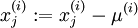
Similarly, $\textstyle u_2^Tx$ is the magnitude of $\textstyle x$ projected onto the vector $\textstyle u_2$ .

Rotating the Data

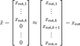
Thus, we can represent $\textstyle x$ in the $\textstyle (u_1, u_2)$ -basis by computing

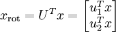
$\begin{align}x_{\rm rot} = U^Tx = \begin{bmatrix} u_1^Tx \\ u_2^Tx \end{bmatrix} \end{align}$

(The subscript "rot" comes from the observation that this corresponds to a rotation (and possibly reflection) of the original data.) Lets take the entire training set, and compute 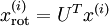$\textstyle x_{\rm rot}^{(i)} = U^Tx^{(i)}$ for every $\textstyle i$ . Plotting this transformed data $\textstyle x_{\rm rot}$ , we get:

This is the training set rotated into the $\textstyle u_1$ , $\textstyle u_2$ basis. In the general case, $\textstyle U^Tx$ will be the training set rotated into the basis $\textstyle u_1$ , $\textstyle u_2$ , ..., $\textstyle u_n$ .

One of the properties of $\textstyle U$ is that it is an "orthogonal" matrix, which means that it satisfies 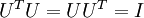$\textstyle U^TU = UU^T = I$ . So if you ever need to go from the rotated vectors $\textstyle x_{\rm rot}$ back to the original data $\textstyle x$ , you can compute

$\begin{align}x = U x_{\rm rot} ,\end{align}$

because $\textstyle U x_{\rm rot} = UU^T x = x$ .

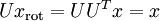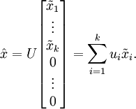
Reducing the Data Dimension

We see that the principal direction of variation of the data is the first dimension $\textstyle x_{{\rm rot},1}$ of this rotated data. Thus, if we want to reduce this data to one dimension, we can set

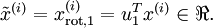
$\begin{align}\tilde{x}^{(i)} = x_{{\rm rot},1}^{(i)} = u_1^Tx^{(i)} \in \Re.\end{align}$

More generally, if $\textstyle x \in \Re^n$ and we want to reduce it to a $\textstyle k$ dimensional representation $\textstyle \tilde{x} \in \Re^k$ (where $\textstyle k < n$ ), we would take the first $\textstyle k$ components of $\textstyle x_{\rm rot}$ , which correspond to the top $\textstyle k$ directions of variation.

Another way of explaining PCA is that $\textstyle x_{\rm rot}$ is an $\textstyle n$ dimensional vector, where the first few components are likely to be large (e.g., in our example, we saw that $\textstyle x_{{\rm rot},1}^{(i)} = u_1^Tx^{(i)}$ takes reasonably large values for most examples $\textstyle i$ ), and the later components are likely to be small (e.g., in our example, $\textstyle x_{{\rm rot},2}^{(i)} = u_2^Tx^{(i)}$ was more likely to be small). What PCA does it it drops the the later (smaller) components of $\textstyle x_{\rm rot}$ , and just approximates them with 0's. Concretely, our definition of $\textstyle \tilde{x}$ can also be arrived at by using an approximation to $\textstyle x_{{\rm rot}}$ where all but the first $\textstyle k$ components are zeros. In other words, we have:

$\begin{align}\tilde{x} = \begin{bmatrix} x_{{\rm rot},1} \\\vdots \\ x_{{\rm rot},k} \\0 \\ \vdots \\ 0 \\ \end{bmatrix}\approx \begin{bmatrix} x_{{\rm rot},1} \\\vdots \\ x_{{\rm rot},k} \\x_{{\rm rot},k+1} \\\vdots \\ x_{{\rm rot},n} \end{bmatrix}= x_{\rm rot} \end{align}$

In our example, this gives us the following plot of $\textstyle \tilde{x}$ (using $\textstyle n=2, k=1$ ):

However, since the final $\textstyle n-k$ components of $\textstyle \tilde{x}$ as defined above would always be zero, there is no need to keep these zeros around, and so we define $\textstyle \tilde{x}$ as a $\textstyle k$ -dimensional vector with just the first $\textstyle k$ (non-zero) components.

This also explains why we wanted to express our data in the $\textstyle u_1, u_2, \ldots, u_n$ basis: Deciding which components to keep becomes just keeping the top $\textstyle k$ components. When we do this, we also say that we are "retaining the top $\textstyle k$ PCA (or principal) components."

Recovering an Approximation of the Data

Now, $\textstyle \tilde{x} \in \Re^k$ is a lower-dimensional, "compressed" representation of the original $\textstyle x \in \Re^n$ . Given $\textstyle \tilde{x}$ , how can we recover an approximation $\textstyle \hat{x}$ to the original value of $\textstyle x$ ? From an earlier section, we know that $\textstyle x = U x_{\rm rot}$ . Further, we can think of $\textstyle \tilde{x}$ as an approximation to $\textstyle x_{\rm rot}$ , where we have set the last $\textstyle n-k$ components to zeros. Thus, given $\textstyle \tilde{x} \in \Re^k$ , we can pad it out with $\textstyle n-k$ zeros to get our approximation to $\textstyle x_{\rm rot} \in \Re^n$ . Finally, we pre-multiply by $\textstyle U$ to get our approximation to $\textstyle x$ . Concretely, we get

$\begin{align}\hat{x} = U \begin{bmatrix} \tilde{x}_1 \\ \vdots \\ \tilde{x}_k \\ 0 \\ \vdots \\ 0 \end{bmatrix} = \sum_{i=1}^k u_i \tilde{x}_i.\end{align}$

The final equality above comes from the definition of $\textstyle U$ given earlier. (In a practical implementation, we wouldn't actually zero pad $\textstyle \tilde{x}$ and then multiply by $\textstyle U$ , since that would mean multiplying a lot of things by zeros; instead, we'd just multiply $\textstyle \tilde{x} \in \Re^k$ with the first $\textstyle k$ columns of $\textstyle U$ as in the final expression above.) Applying this to our dataset, we get the following plot for $\textstyle \hat{x}$ :

We are thus using a 1 dimensional approximation to the original dataset.

If you are training an autoencoder or other unsupervised feature learning algorithm, the running time of your algorithm will depend on the dimension of the input. If you feed $\textstyle \tilde{x} \in \Re^k$ into your learning algorithm instead of $\textstyle x$ , then you'll be training on a lower-dimensional input, and thus your algorithm might run significantly faster. For many datasets, the lower dimensional $\textstyle \tilde{x}$ representation can be an extremely good approximation to the original, and using PCA this way can significantly speed up your algorithm while introducing very little approximation error.

Number of components to retain

How do we set $\textstyle k$ ; i.e., how many PCA components should we retain? In our simple 2 dimensional example, it seemed natural to retain 1 out of the 2 components, but for higher dimensional data, this decision is less trivial. If $\textstyle k$ is too large, then we won't be compressing the data much; in the limit of $\textstyle k=n$ , then we're just using the original data (but rotated into a different basis). Conversely, if $\textstyle k$ is too small, then we might be using a very bad approximation to the data.

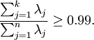
To decide how to set $\textstyle k$ , we will usually look at the percentage of variance retained for different values of $\textstyle k$ . Concretely, if $\textstyle k=n$ , then we have an exact approximation to the data, and we say that 100% of the variance is retained. I.e., all of the variation of the original data is retained. Conversely, if $\textstyle k=0$ , then we are approximating all the data with the zero vector, and thus 0% of the variance is retained.

More generally, let $\textstyle \lambda_1, \lambda_2, \ldots, \lambda_n$ be the eigenvalues of $\textstyle \Sigma$ (sorted in decreasing order), so that $\textstyle \lambda_j$ is the eigenvalue corresponding to the eigenvector $\textstyle u_j$ . Then if we retain $\textstyle k$ principal components, the percentage of variance retained is given by:

$\begin{align}\frac{\sum_{j=1}^k \lambda_j}{\sum_{j=1}^n \lambda_j}.\end{align}$

In our simple 2D example above, $\textstyle \lambda_1 = 7.29$ , and $\textstyle \lambda_2 = 0.69$ . Thus, by keeping only $\textstyle k=1$ principal components, we retained $\textstyle 7.29/(7.29+0.69) = 0.913$ , or 91.3% of the variance.

A more formal definition of percentage of variance retained is beyond the scope of these notes. However, it is possible to show that 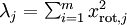$\textstyle \lambda_j =\sum_{i=1}^m x_{{\rm rot},j}^2$ . Thus, if $\textstyle \lambda_j \approx 0$ , that shows that $\textstyle x_{{\rm rot},j}$ is usually near 0 anyway, and we lose relatively little by approximating it with a constant 0. This also explains why we retain the top principal components (corresponding to the larger values of $\textstyle \lambda_j$ ) instead of the bottom ones. The top principal components $\textstyle x_{{\rm rot},j}$ are the ones that're more variable and that take on larger values, and for which we would incur a greater approximation error if we were to set them to zero.

In the case of images, one common heuristic is to choose $\textstyle k$ so as to retain 99% of the variance. In other words, we pick the smallest value of $\textstyle k$ that satisfies

$\begin{align}\frac{\sum_{j=1}^k \lambda_j}{\sum_{j=1}^n \lambda_j} \geq 0.99. \end{align}$

Depending on the application, if you are willing to incur some additional error, values in the 90-98% range are also sometimes used. When you describe to others how you applied PCA, saying that you chose $\textstyle k$ to retain 95% of the variance will also be a much more easily interpretable description than saying that you retained 120 (or whatever other number of) components.

PCA on Images

For PCA to work, usually we want each of the features $\textstyle x_1, x_2, \ldots, x_n$ to have a similar range of values to the others (and to have a mean close to zero). If you've used PCA on other applications before, you may therefore have separately pre-processed each feature to have zero mean and unit variance, by separately estimating the mean and variance of each feature $\textstyle x_j$ . However, this isn't the pre-processing that we will apply to most types of images. Specifically, suppose we are training our algorithm on natural images, so that $\textstyle x_j$ is the value of pixel $\textstyle j$ . By "natural images," we informally mean the type of image that a typical animal or person might see over their lifetime.

Note: Usually we use images of outdoor scenes with grass, trees, etc., and cut out small (say 16x16) image patches randomly from these to train the algorithm. But in practice most feature learning algorithms are extremely robust to the exact type of image it is trained on, so most images taken with a normal camera, so long as they aren't excessively blurry or have strange artifacts, should work.

When training on natural images, it makes little sense to estimate a separate mean and variance for each pixel, because the statistics in one part of the image should (theoretically) be the same as any other. This property of images is calledstationarity.

In detail, in order for PCA to work well, informally we require that (i) The features have approximately zero mean, and (ii) The different features have similar variances to each other. With natural images, (ii) is already satisfied even without variance normalization, and so we won't perform any variance normalization. (If you are training on audio data---say, on spectrograms---or on text data---say, bag-of-word vectors---we will usually not perform variance normalization either.) In fact, PCA is invariant to the scaling of the data, and will return the same eigenvectors regardless of the scaling of the input. More formally, if you multiply each feature vector $\textstyle x$ by some positive number (thus scaling every feature in every training example by the same number), PCA's output eigenvectors will not change.

So, we won't use variance normalization. The only normalization we need to perform then is mean normalization, to ensure that the features have a mean around zero. Depending on the application, very often we are not interested in how bright the overall input image is. For example, in object recognition tasks, the overall brightness of the image doesn't affect what objects there are in the image. More formally, we are not interested in the mean intensity value of an image patch; thus, we can subtract out this value, as a form of mean normalization.

Concretely, if $\textstyle x^{(i)} \in \Re^{n}$ are the (grayscale) intensity values of a 16x16 image patch ( $\textstyle n=256$ ), we might normalize the intensity of each image $\textstyle x^{(i)}$ as follows:

$\mu^{(i)} := \frac{1}{n} \sum_{j=1}^n x^{(i)}_j$

$x^{(i)}_j := x^{(i)}_j - \mu^{(i)}$ , for all $\textstyle j$

Note that the two steps above are done separately for each image $\textstyle x^{(i)}$ , and that $\textstyle \mu^{(i)}$ here is the mean intensity of the image $\textstyle x^{(i)}$ . In particular, this is not the same thing as estimating a mean value separately for each pixel $\textstyle x_j$ .

If you are training your algorithm on images other than natural images (for example, images of handwritten characters, or images of single isolated objects centered against a white background), other types of normalization might be worth considering, and the best choice may be application dependent. But when training on natural images, using the per-image mean normalization method as given in the equations above would be a reasonable default.

jingruixiaozhuang

关注

0
点赞
踩
0

收藏

觉得还不错? 一键收藏
0
评论
Deep learning------------PCA (principle component analysis)

PCA在 stanford CS229课程里有详细的讲解：一下是对PCA从各个方面的深入剖析：IntroductionPrincipal Components Analysis (PCA) is a dimensionality reduction algorithm that can be used to significantly speed up yo
复制链接

扫一扫