


Non-Maximum Suppression for Object Detection in Python
Connecticut is cold. Very cold. Sometimes it’s hard to even get out of bed in the morning. And honestly, without the aide of copious amounts of pumpkin spice lattes and the beautiful sunrise over the crisp autumn leaves, I don’t think I would leave my cozy bed.
But I have work to do. And today that work includes writing a blog post about Felzenszwalb et al. method for non-maximum suppression.
If you remember, last week we discussed Histogram of Oriented Gradients for Objection Detection.
This method can be broken into a 6-step process, including:
- Sampling positive images
- Sampling negative images
- Training a Linear SVM
- Performing hard-negative mining
- Re-training your Linear SVM using the hard-negative samples
- Evaluating your classifier on your test dataset, utilizing non-maximum suppression to ignore redundant, overlapping bounding boxes
After applying these steps you’ll have an object detector that is as smooth as, well, John Coltrane:
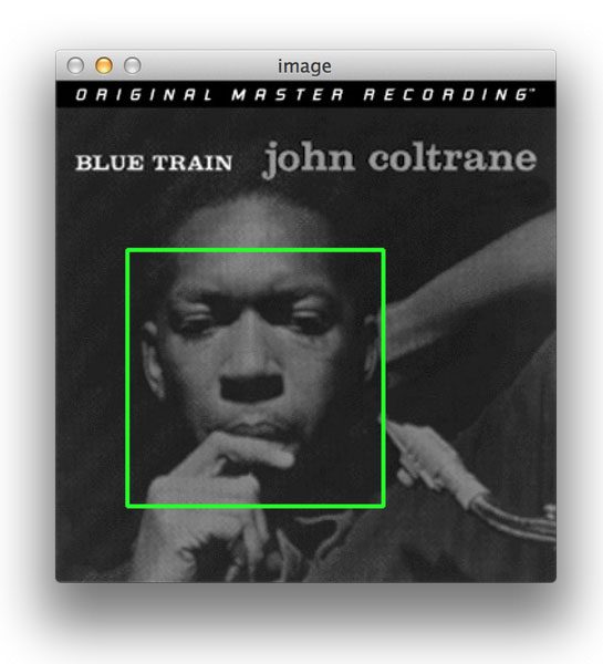
Figure 1: My Python object detection framework applied to face detection. Even in low contrast images, faces can be easily detected.
(Note: Images utilized in this post were taken from the MIT + CMU Frontal Face Images dataset)
These are the bare minimum steps required to build an object classifier using Histogram of Oriented Gradients. Extensions to this method exist including Felzenszwalb et al.’s deformable parts model and Malisiewicz et al.’s Exemplar SVM.
However, no matter which HOG + Linear SVM method you choose, you will (with almost 100% certainty) detect multiple bounding boxes surrounding the object in the image.
For example, take a look at the image of Audrey Hepburn at the top of this post. I forked my Python framework for object detection using HOG and a Linear SVM and trained it to detect faces. Clearly, it has found Ms. Hepburns face in the image — but the detection fired a total of six times!
While each detection may in fact be valid, I certainty don’t want my classifier to report to back to me saying that it found six faces when there is clearly only one face. Like I said, this is common “problem” when utilizing object detection methods.
In fact, I don’t even want to call it a “problem” at all! It’s a good problem to have. It indicates that your detector is working as expected. It would be far worse if your detector either (1) reported a false positive (i.e. detected a face where one wasn’t) or (2) failed to detect a face.
To fix this situation we’ll need to apply Non-Maximum Suppression (NMS), also called Non-Maxima Suppression.
When I first implemented my Python object detection framework I was unaware of a good Python implementation for Non-Maximum Suppression, so I reached out to my friend Dr. Tomasz Malisiewicz, whom I consider to be the “go to” person on the topic of object detection and HOG.
Tomasz, being the all-knowing authority on the topic referred me to two implementations in MATLAB which I have since implemented in Python. We’re going to review the first method by Felzenszwalb etl al. Then, next week, we’ll review the (faster) non-maximum suppression method implemented by Tomasz himself.
So without very delay, let’s get our hands dirty.
Looking for the source code to this post?
Jump right to the downloads section.
OpenCV and Python versions:
This example will run on Python 2.7/Python 3.4+ and OpenCV 2.4.X/OpenCV 3.0+.
Non-Maximum Suppression for Object Detection in Python
Open up a file, name it nms.py , and let’s get started implementing the Felzenszwalb et al. method for non-maximum suppression in Python:
We’ll start on Line 2 by importing a single package, NumPy, which we’ll utilize for numerical processing.
From there we define our non_max_suppression_slow function on Line 5. this function accepts to arguments, the first being our set of bounding boxes in the form of (startX, startY, endX, endY) and the second being our overlap threshold. I’ll discuss the overlap threshold a little later on in this post.
Lines 7 and 8 make a quick check on the bounding boxes. If there are no bounding boxes in the list, simply return an empty list back to the caller.
From there, we initialize our list of picked bounding boxes (i.e. the bounding boxes that we would like to keep, discarding the rest) on Line 11.
Let’s go ahead and unpack the (x, y) coordinates for each corner of the bounding box on Lines 14-17 — this is done using simple NumPy array slicing.
Then we compute the area of each of the bounding boxes on Line 21 using our sliced (x, y)coordinates.
Be sure to pay close attention to Line 22. We apply np.argsort to grab the indexes of the sorted coordinates of the bottom-right y-coordinate of the bounding boxes. It is absolutely critical that we sort according to the bottom-right corner as we’ll need to compute the overlap ratio of other bounding boxes later in this function.
Now, let’s get into the meat of the non-maxima suppression function:
We start looping over our indexes on Line 26, where we will keep looping until we run out of indexes to examine.
From there we’ll grab the length of the idx list o Line 31, grab the value of the last entry in theidx list on Line 32, append the index i to our list of bounding boxes to keep on Line 33, and finally initialize our suppress list (the list of boxes we want to ignore) with index of the last entry of the index list on Line 34.
That was a mouthful. And since we’re dealing with indexes into a index list it’s not exactly an easy thing to explain. But definitely pause here and examine these code as it’s important to understand.
Time to compute the overlap ratios and determine which bounding boxes we can ignore:
Here we start looping over the (remaining) indexes in the idx list on Line 37, grabbing the value of the current index on Line 39.
Using last entry in the idx list from Line 32 and the current entry in the idx list from Line 39, we find the largest (x, y) coordinates for the start bounding box and the smallest (x, y)coordinates for the end of the bounding box on Lines 44-47.
Doing this allows us to find the current smallest region inside the larger bounding boxes (and hence why it’s so important that we initially sort our idx list according to the bottom-right y-coordinate). From there, we compute the width and height of the region on Lines 50 and 51.
So now we are at the point where the overlap threshold comes into play. On Line 55 we compute the overlap , which is a ratio defined by the area of the current smallest region divided by the area of current bounding box, where “current” is defined by the index j on Line 39.
If the overlap ratio is greater than the threshold on Line 59, then we know that the two bounding boxes sufficiently overlap and we can thus suppress the current bounding box. Common values for overlapThresh are normally between 0.3 and 0.5.
Line 64 then deletes the suppressed bounding boxes from the idx list and we continue looping until the idx list is empty.
Finally, we return the set of picked bounding boxes (the ones that were not suppressed) on Line 67.
Let’s go ahead and create a driver so we can execute this code and see it in action. Open up a new file, name it nms_slow.py , and add the following code:
We start by importing our non_max_suppression_slow function on Line 2. I put this function in the pyimagesearch package for organizational purposes, but you can put the function wherever you see fit. From there, we import NumPy for numerical processing and cv2 for our OpenCV bindings on Lines 3-4.
Then, we define a list of images on Line 8. This list consists of 2-tuples, where the first entry in the tuple is a path to an image and the second entry is the list of bounding boxes. These bounding boxes were obtained from my HOG + Linear SVM classifier detecting potential “faces” at varying locations and scales. Our goal is to take the set of bounding boxes for each image and apply non-maximum suppression.
We start by looping over the image path and bounding boxes on Line 27 and load the image on Line 30.
To visualize the results of non-maximum suppression in action, we first draw the original (non-suppressed) bounding boxes on Lines 34 and 35.
We then apply non-maximum suppression on Line 38 and draw the picked bounding boxes on Lines 42-43.
The resulting images are finally displayed on Lines 46-48.
Non-Maximum Suppression in Action
To see the Felzenszwalb et al. non-maximum suppression method in action, download the source code and accompanying images for this post from the bottom of this page, navigate to the source code directory, and issue the following command:
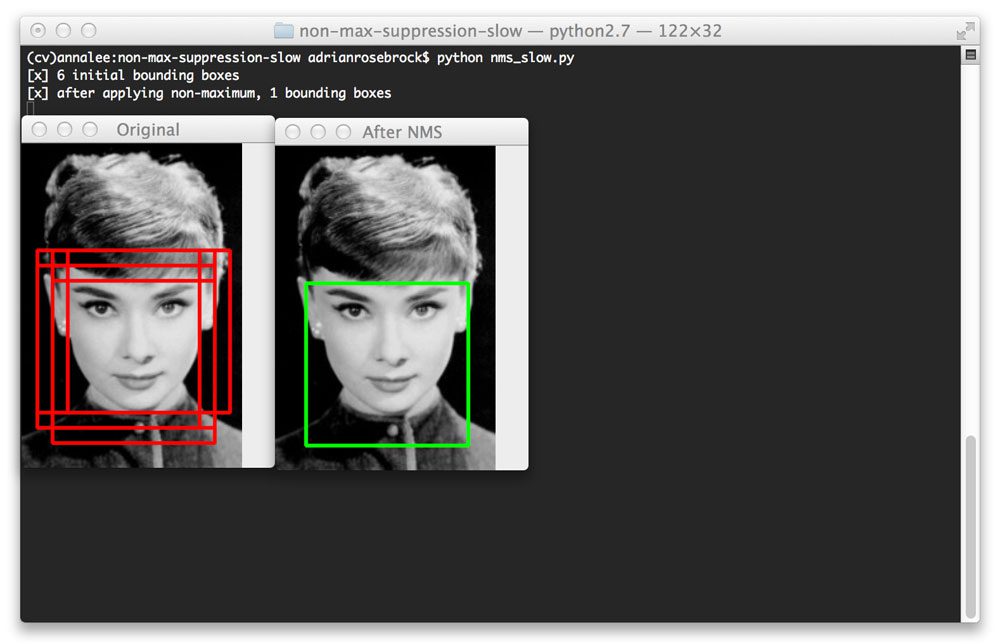
First, you’ll see the Audrey Hepburn image:
Figure 2: Our classifier initially detected six bounding boxes, but by applying non-maximum suppression, we are left with only one (the correct) bounding box.
Notice how six bounding boxes were detected, but by applying non-maximum suppression, we are able to prune this number down to one.
The same is true for the second image:
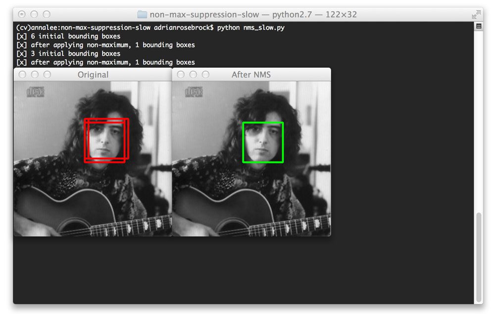
Figure 3: Initially detecting three bounding boxes, but by applying non-maximum suppression we can prune the number of overlapping bounding boxes down to one.
Here we have found three bounding boxes corresponding to the same face, but non-maximum suppression is about to reduce this number to one bounding box.
So far we have only examined images that contain one face. But what about images that contain multiple faces? Let’s take a look:
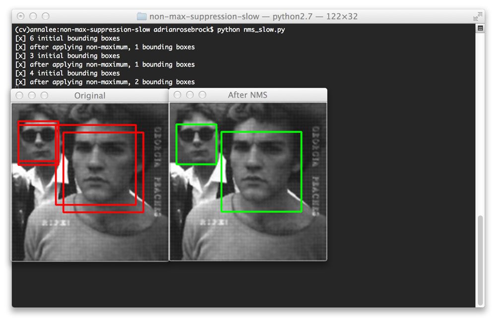
Figure 4: Non-maximum suppression correctly handles when there are multiple faces, suppressing the smaller overlapping bounding boxes, but retaining the boxes that do not overlap.
Even for images that contain multiple objects, non-maximum suppression is able to ignore the smaller overlapping bounding boxes and return only the larger ones. Non-maximum suppression returns two bounding boxes here because the bounding boxes for each face at all. And even if they did overlap, do the overlap ratio does not exceed the supplied threshold of 0.3.
Summary
In this blog post I showed you how to apply the Felzenszwalb et al. method for non-maximum suppression.
When using the Histogram of Oriented Gradients descriptor and a Linear Support Vector Machine for object classification you almost always detect multiple bounding boxes surrounding the object you want to detect.
Instead of returning all of the found bounding boxes you should first apply non-maximum suppression to ignore bounding boxes that significantly overlap each other.
However, there are improvements to be made to the Felzenszwalb et al. method for non-maximum suppression.
In my next post I’ll implement the method suggested by my friend Dr. Tomasz Malisiewicz which is reported to be over 100x faster!
Be sure to download the code to this post using the form below! You’ll definitely want to have it handy when we examine Tomasz’s non-maximum suppression algorithm next week!
Downloads:
Resource Guide (it’s totally free).


 1075
1075


 被折叠的 条评论
为什么被折叠?
被折叠的 条评论
为什么被折叠?
 到【灌水乐园】发言


