


Numpy
Numpy是Python科学计算的核心库。它提供了高性能多维数组对象,以及使用这些数组的工具。如果你已经熟悉MATLAB,你可以找到这个教程来开始使用Numpy。
Arrays
一个numpy的数组(array)是一个由相同类型数值构成的网络(grid),并且被非负整数的元组索引。维数是数组的rank;而数组的shape是一个整数元组,它给出了数组每一维度的大小。
我们可以使用嵌套的Python lists初始化numpy数组,并使用方括号来访问元素。
import numpy as np

a = np.array([1, 2, 3])  # Create a rank 1 array
print type(a)            # Prints "<type 'numpy.ndarray'>"
print a.shape            # Prints "(3,)"
print a[0], a[1], a[2]   # Prints "1 2 3"
a[0] = 5                 # Change an element of the array
print a                  # Prints "[5, 2, 3]"

b = np.array([[1,2,3],[4,5,6]])   # Create a rank 2 array
print b.shape                     # Prints "(2, 3)"
print b[0, 0], b[0, 1], b[1, 0]   # Prints "1 2 4"
Numpy也提供了很多函数来创建数组。
import numpy as np

a = np.zeros((2,2))  # Create an array of all zeros
print a              # Prints "[[ 0.  0.]
                     #          [ 0.  0.]]"

b = np.ones((1,2))   # Create an array of all ones
print b              # Prints "[[ 1.  1.]]"

c = np.full((2,2), 7) # Create a constant array
print c               # Prints "[[ 7.  7.]
                      #          [ 7.  7.]]"

d = np.eye(2)        # Create a 2x2 identity matrix
print d              # Prints "[[ 1.  0.]
                     #          [ 0.  1.]]"

e = np.random.random((2,2)) # Create an array filled with random values
print e                     # Might print "[[ 0.91940167  0.08143941]
                            #               [ 0.68744134  0.87236687]]"
你可以在官方文档中找到更多的数组创建的方法。
Array indexing
Numpy提供了一些方法来索引数组。
Slicing:与Python lists类似,numpy 数组可以被切分。数组可能是多维的,你必须为每一维度确定一个切分。
import numpy as np

# Create the following rank 2 array with shape (3, 4)
# [[ 1  2  3  4]
#  [ 5  6  7  8]
#  [ 9 10 11 12]]
a = np.array([[1,2,3,4], [5,6,7,8], [9,10,11,12]])

# Use slicing to pull out the subarray consisting of the first 2 rows
# and columns 1 and 2; b is the following array of shape (2, 2):
# [[2 3]
#  [6 7]]
b = a[:2, 1:3]

# A slice of an array is a view into the same data, so modifying it
# will modify the original array.
print a[0, 1]   # Prints "2"
b[0, 0] = 77    # b[0, 0] is the same piece of data as a[0, 1]
print a[0, 1]   # Prints "77"
你可以混合使用整数索引和切分索引。然而,这样做会产生一个低阶的数组。这与MATLAB中操作数组切分的方式是完全不同的。
import numpy as np

# Create the following rank 2 array with shape (3, 4)
# [[ 1  2  3  4]
#  [ 5  6  7  8]
#  [ 9 10 11 12]]
a = np.array([[1,2,3,4], [5,6,7,8], [9,10,11,12]])

# Two ways of accessing the data in the middle row of the array.
# Mixing integer indexing with slices yields an array of lower rank,
# while using only slices yields an array of the same rank as the
# original array:
row_r1 = a[1, :]    # Rank 1 view of the second row of a
row_r2 = a[1:2, :]  # Rank 2 view of the second row of a
print row_r1, row_r1.shape  # Prints "[5 6 7 8] (4,)"
print row_r2, row_r2.shape  # Prints "[[5 6 7 8]] (1, 4)"

# We can make the same distinction when accessing columns of an array:
col_r1 = a[:, 1]
col_r2 = a[:, 1:2]
print col_r1, col_r1.shape  # Prints "[ 2  6 10] (3,)"
print col_r2, col_r2.shape  # Prints "[[ 2]
                            #          [ 6]
                            #          [10]] (3, 1)"
Integerarray indexing: 当使用slicing索引到numpy 数组内部的时候,所得的数组是原始数组的子数组。相反,整数形式的数组索引允许你使用其他数组的数据来创建任意数组。示例如下:
import numpy as np

a = np.array([[1,2], [3, 4], [5, 6]])

# An example of integer array indexing.
# The returned array will have shape (3,) and
print a[[0, 1, 2], [0, 1, 0]]  # Prints "[1 4 5]"

# The above example of integer array indexing is equivalent to this:
print np.array([a[0, 0], a[1, 1], a[2, 0]])  # Prints "[1 4 5]"

# When using integer array indexing, you can reuse the same
# element from the source array:
print a[[0, 0], [1, 1]]  # Prints "[2 2]"

# Equivalent to the previous integer array indexing example
print np.array([a[0, 1], a[0, 1]])  # Prints "[2 2]"
关于整数索引的一个有用的技巧是选择或者改变来自矩阵每行的一个元素。
import numpy as np

# Create a new array from which we will select elements
a = np.array([[1,2,3], [4,5,6], [7,8,9], [10, 11, 12]])

print a  # prints "array([[ 1,  2,  3],
         #                [ 4,  5,  6],
         #                [ 7,  8,  9],
         #                [10, 11, 12]])"

# Create an array of indices
b = np.array([0, 2, 0, 1])

# Select one element from each row of a using the indices in b
print a[np.arange(4), b]  # Prints "[ 1  6  7 11]"

# Mutate one element from each row of a using the indices in b
a[np.arange(4), b] += 10

print a  # prints "array([[11,  2,  3],
         #                [ 4,  5, 16],
         #                [17,  8,  9],
         #                [10, 21, 12]])
Booleanarray indexing: 布尔型数组索引允许你挑选出数组的任意元素。这种索引方式用于选择数组中满足特定条件的元素。示例如下:
import numpy as np

a = np.array([[1,2], [3, 4], [5, 6]])

bool_idx = (a > 2)  # Find the elements of a that are bigger than 2;
                    # this returns a numpy array of Booleans of the same
                    # shape as a, where each slot of bool_idx tells
                    # whether that element of a is > 2.

print bool_idx      # Prints "[[False False]
                    #          [ True  True]
                    #          [ True  True]]"

# We use boolean array indexing to construct a rank 1 array
# consisting of the elements of a corresponding to the True values
# of bool_idx
print a[bool_idx]  # Prints "[3 4 5 6]"

# We can do all of the above in a single concise statement:
print a[a > 2]     # Prints "[3 4 5 6]"
为了简洁,关于numpy数组索引的很多细节没有介绍;如果想了解更多,可以阅读官方文档。
Datatypes
每一个numpy数组是一个由相同类型元素组成的网络。Numpy提供大量的数值类型,你可以用它们来构建数组。在你创建数组时候,Numpy尝试猜测数据类型,但是创建数组的函数通常会包含一个可选的参数来确定数据类型。这里有一个示例:
import numpy as np

x = np.array([1, 2])  # Let numpy choose the datatype
print x.dtype         # Prints "int64"

x = np.array([1.0, 2.0])  # Let numpy choose the datatype
print x.dtype             # Prints "float64"

x = np.array([1, 2], dtype=np.int64)  # Force a particular datatype
print x.dtype                         # Prints "int64"
你也可以在官方文档中阅读所有的numpy数据类型。
Array math
基本的数学函数在数组上进行元素级操作,在运算符重载和numpy模块的函数中都是可用的:
import numpy as np

x = np.array([[1,2],[3,4]], dtype=np.float64)
y = np.array([[5,6],[7,8]], dtype=np.float64)

# Elementwise sum; both produce the array
# [[ 6.0  8.0]
#  [10.0 12.0]]
print x + y
print np.add(x, y)

# Elementwise difference; both produce the array
# [[-4.0 -4.0]
#  [-4.0 -4.0]]
print x - y
print np.subtract(x, y)

# Elementwise product; both produce the array
# [[ 5.0 12.0]
#  [21.0 32.0]]
print x * y
print np.multiply(x, y)

# Elementwise division; both produce the array
# [[ 0.2         0.33333333]
#  [ 0.42857143  0.5       ]]
print x / y
print np.divide(x, y)

# Elementwise square root; produces the array
# [[ 1.          1.41421356]
#  [ 1.73205081  2.        ]]
print np.sqrt(x)
注意,与MATLAB中不同,“*”表示元素乘法,不是矩阵乘法。我们使用dot函数来计算向量内积,向量与矩阵相乘,已经矩阵乘法。dot 既可以作为numpy模块中的一个函数,也可以作为数组对象的一个示例方法:
import numpy as np

x = np.array([[1,2],[3,4]])
y = np.array([[5,6],[7,8]])

v = np.array([9,10])
w = np.array([11, 12])

# Inner product of vectors; both produce 219
print v.dot(w)
print np.dot(v, w)

# Matrix / vector product; both produce the rank 1 array [29 67]
print x.dot(v)
print np.dot(x, v)

# Matrix / matrix product; both produce the rank 2 array
# [[19 22]
#  [43 50]]
print x.dot(y)
print np.dot(x, y)
Numpy提供了很多有用的函数来在数组上做运算;最有用的一个是sum:
import numpy as np

x = np.array([[1,2],[3,4]])

print np.sum(x)  # Compute sum of all elements; prints "10"
print np.sum(x, axis=0)  # Compute sum of each column; prints "[4 6]"
print np.sum(x, axis=1)  # Compute sum of each row; prints "[3 7]"
你可以在官方文档中找到numpy提供的数学函数的列表。
除了在数学函数中使用数组,我们经常还会需要对数组中的数据进行操作或者重构。这种操作最简单的例子就是转置一个矩阵;要转置一个矩阵,可以使用数组对象的T属性。
import numpy as np

x = np.array([[1,2], [3,4]])
print x    # Prints "[[1 2]
           #          [3 4]]"
print x.T  # Prints "[[1 3]
           #          [2 4]]"

# Note that taking the transpose of a rank 1 array does nothing:
v = np.array([1,2,3])
print v    # Prints "[1 2 3]"
print v.T  # Prints "[1 2 3]"
Numpy提供了非常多的操作数组的函数;你可以在官方文档中找到它们。
Broadcasting
广播是一个强大的机制,它允许numpy在进行算数操作的时候可以使用不同的形状的数组。经常会有这种情况,我们有一个小数组和一个大数组,我们相用小数组多次在大数组上进行操作。
例如,设想我们要往矩阵的每一行上加一个常数向量。我们可以这样做:
import numpy as np

# We will add the vector v to each row of the matrix x,
# storing the result in the matrix y
x = np.array([[1,2,3], [4,5,6], [7,8,9], [10, 11, 12]])
v = np.array([1, 0, 1])
y = np.empty_like(x)   # Create an empty matrix with the same shape as x

# Add the vector v to each row of the matrix x with an explicit loop
for i in range(4):
    y[i, :] = x[i, :] + v

# Now y is the following
# [[ 2  2  4]
#  [ 5  5  7]
#  [ 8  8 10]
#  [11 11 13]]
print y
这是可以正常工作的;但是当矩阵x非常大的时候,计算一个显式循环在Python中是非常慢的。须知,将一个向量v加到矩阵x的每一行上,等效于通过垂直存储v的多个副本来构建一个矩阵vv,然后对x和vv执行元素级求和。我们可以这样执行这个方法:
import numpy as np

# We will add the vector v to each row of the matrix x,
# storing the result in the matrix y
x = np.array([[1,2,3], [4,5,6], [7,8,9], [10, 11, 12]])
v = np.array([1, 0, 1])
vv = np.tile(v, (4, 1))  # Stack 4 copies of v on top of each other
print vv                 # Prints "[[1 0 1]
                         #          [1 0 1]
                         #          [1 0 1]
                         #          [1 0 1]]"
y = x + vv  # Add x and vv elementwise
print y  # Prints "[[ 2  2  4
         #          [ 5  5  7]
         #          [ 8  8 10]
         #          [11 11 13]]"
Numpy广播允许我们执行这个操作,但是不必真得创建v的多个副本。考虑使用广播的版本:
import numpy as np

# We will add the vector v to each row of the matrix x,
# storing the result in the matrix y
x = np.array([[1,2,3], [4,5,6], [7,8,9], [10, 11, 12]])
v = np.array([1, 0, 1])
y = x + v  # Add v to each row of x using broadcasting
print y  # Prints "[[ 2  2  4]
         #          [ 5  5  7]
         #          [ 8  8 10]
         #          [11 11 13]]"
即使x的shape是(4,3),而v的shape是(3,),y = x + v 仍然可以工作,这多亏了广播;这一行工作时好像v的shape是(4,3),每一行是v的一个副本,求和是以元素级别执行的。
一起广播两个数组遵循这些规则:
(1) 如果数组没有相同的阶数,预先考虑低阶数组,直到两个shapes有相同的长度。
(2) 如果他们在一个维度上具有相同的尺寸,或者其中一个在该维度上的size是1,就说它们是兼容的。
(3)如果它们在所有的维度上是兼容的,就可以一起广播。
(4) 广播后,每一个数组的shape表现得像是与两个数组的shape中最大那个元素相同。
(5) 在任何一个维度,如果一个数组的size是1,而另一个大于1,则第一个数组表现得像是在该维度上进行了拷贝。
支持广播的函数成为通用函数。你可以在官方文档中找到通用函数的列表。
这里是关于广播的一些应用:import numpy as np
# Compute outer product of vectors
v = np.array([1,2,3]) # v has shape (3,)
w = np.array([4,5]) # w has shape (2,)
# To compute an outer product, we first reshape v to be a column
# vector of shape (3, 1); we can then broadcast it against w to yield
# an output of shape (3, 2), which is the outer product of v and w:
# [[ 4 5]
# [ 8 10]
# [12 15]]
print np.reshape(v, (3, 1)) * w
# Add a vector to each row of a matrix
x = np.array([[1,2,3], [4,5,6]])
# x has shape (2, 3) and v has shape (3,) so they broadcast to (2, 3),
# giving the following matrix:
# [[2 4 6]
# [5 7 9]]
print x + v
# Add a vector to each column of a matrix
# x has shape (2, 3) and w has shape (2,).
# If we transpose x then it has shape (3, 2) and can be broadcast
# against w to yield a result of shape (3, 2); transposing this result
# yields the final result of shape (2, 3) which is the matrix x with
# the vector w added to each column. Gives the following matrix:
# [[ 5 6 7]
# [ 9 10 11]]
print (x.T + w).T
# Another solution is to reshape w to be a row vector of shape (2, 1);
# we can then broadcast it directly against x to produce the same
# output.
print x + np.reshape(w, (2, 1))
# Multiply a matrix by a constant:
# x has shape (2, 3). Numpy treats scalars as arrays of shape ();
# these can be broadcast together to shape (2, 3), producing the
# following array:
# [[ 2 4 6]
# [ 8 10 12]]
print x * 2
广播能够使代码更加简洁和快速,你应该在可能的地方尽量使用它。
Numpy Documentation
这个简要的概述涉及了很多你应该了解的关于numpy的重要内容,但是远远不够完整。查看Numpy索引来找到更多的关于Numpy的内容。
Scipy
Numpy提供了一个高性能多维度数组和计算、操作这些数组的基本工具。SciPy在此基础上构建而成,提供大量的在numpy数组上操作的函数,可以用于不同类型的科学和工程应用。
最好的熟悉SciPy的方式是浏览文档。我们会重点强调一些对本课程有用的部分。
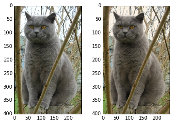
Image operations
SciPy提供了一些基本的函数来处理图像。例如,把图像从硬盘读入numpy数组,将numpy数组以图像格式写到硬盘,重新设置图像的大小。示例如下:from scipy.misc import imread, imsave, imresize
# Read an JPEG image into a numpy array
img = imread('assets/cat.jpg')
print img.dtype, img.shape # Prints "uint8 (400, 248, 3)"
# We can tint the image by scaling each of the color channels
# by a different scalar constant. The image has shape (400, 248, 3);
# we multiply it by the array [1, 0.95, 0.9] of shape (3,);
# numpy broadcasting means that this leaves the red channel unchanged,
# and multiplies the green and blue channels by 0.95 and 0.9
# respectively.
img_tinted = img * [1, 0.95, 0.9]
# Resize the tinted image to be 300 by 300 pixels.
img_tinted = imresize(img_tinted, (300, 300))
# Write the tinted image back to disk
imsave('assets/cat_tinted.jpg', img_tinted)
---------------------------------------------------------------------------------------


Left: The original image. Right: The tintedand resized image.
---------------------------------------------------------------------------------------
MATLAB files
函数scipy.io.loadmat 和 scipy.io.savemat 允许你读写MATLAB文件,你可以从官方文档中了解到它们。
Distance between points
SciPy定义了一些有用的函数来计算点之间的距离。
函数scipy.spatial.distance.pdist 计算给定集合中所有点对的距离。
import numpy as np
from scipy.spatial.distance import pdist, squareform

# Create the following array where each row is a point in 2D space:
# [[0 1]
#  [1 0]
#  [2 0]]
x = np.array([[0, 1], [1, 0], [2, 0]])
print x

# Compute the Euclidean distance between all rows of x.
# d[i, j] is the Euclidean distance between x[i, :] and x[j, :],
# and d is the following array:
# [[ 0.          1.41421356  2.23606798]
#  [ 1.41421356  0.          1.        ]
#  [ 2.23606798  1.          0.        ]]
d = squareform(pdist(x, 'euclidean'))
print d
你可以从官网文档中获取该函数更多的细节。
一个类似的函数(scipy.spatial.distance.cdist)计算两个集合中所有点对之间的距离;你可以在这里阅读它们。
Matplotlib
Matplotlib是一个绘图库。这个部分主要介绍matplotlib.pyplot模块,它提供了一个与MATLAB类型的绘图系统。
Plotting
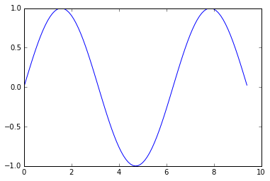
matplotlib中最重要的函数是plot,它让我们可以绘制2D数据。这有一个简单的例子:
import numpy as np
import matplotlib.pyplot as plt

# Compute the x and y coordinates for points on a sine curve
x = np.arange(0, 3 * np.pi, 0.1)
y = np.sin(x)

# Plot the points using matplotlib
plt.plot(x, y)
plt.show()  # You must call plt.show() to make graphics appear.
运行代码可以获得下面的图形。
-------------------------------------------------------------------------------------------
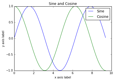
做一点额外的工作,我们就能一次绘制多条线,添加标题、图例和坐标轴标签。
import numpy as np
import matplotlib.pyplot as plt

# Compute the x and y coordinates for points on sine and cosine curves
x = np.arange(0, 3 * np.pi, 0.1)
y_sin = np.sin(x)
y_cos = np.cos(x)

# Plot the points using matplotlib
plt.plot(x, y_sin)
plt.plot(x, y_cos)
plt.xlabel('x axis label')
plt.ylabel('y axis label')
plt.title('Sine and Cosine')
plt.legend(['Sine', 'Cosine'])
plt.show()
-------------------------------------------------------------------------------------------
-------------------------------------------------------------------------------------------
你可以在官方文档中阅读到更多的关于plot的内容。
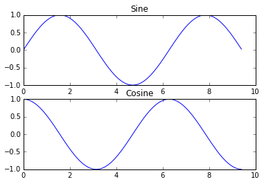
Subplots
可以在同一个图中绘制不同的东西,需要使用subplot函数。这里是一个例子:
import numpy as np
import matplotlib.pyplot as plt

# Compute the x and y coordinates for points on sine and cosine curves
x = np.arange(0, 3 * np.pi, 0.1)
y_sin = np.sin(x)
y_cos = np.cos(x)

# Set up a subplot grid that has height 2 and width 1,
# and set the first such subplot as active.
plt.subplot(2, 1, 1)

# Make the first plot
plt.plot(x, y_sin)
plt.title('Sine')

# Set the second subplot as active, and make the second plot.
plt.subplot(2, 1, 2)
plt.plot(x, y_cos)
plt.title('Cosine')

# Show the figure.
plt.show()
-------------------------------------------------------------------------------------------
-------------------------------------------------------------------------------------------
同样,官方文档提供了更多的关于subplot的内容。
Images
你可以使用imshow函数来展示图片。示例如下:
import numpy as np
from scipy.misc import imread, imresize
import matplotlib.pyplot as plt

img = imread('assets/cat.jpg')
img_tinted = img * [1, 0.95, 0.9]

# Show the original image
plt.subplot(1, 2, 1)
plt.imshow(img)

# Show the tinted image
plt.subplot(1, 2, 2)

# A slight gotcha with imshow is that it might give strange results
# if presented with data that is not uint8. To work around this, we
# explicitly cast the image to uint8 before displaying it.
plt.imshow(np.uint8(img_tinted))
plt.show()
-------------------------------------------------------------------------------------------
-------------------------------------------------------------------------------------------


 被折叠的 条评论
为什么被折叠?
被折叠的 条评论
为什么被折叠?
 到【灌水乐园】发言


