线性回归 numpy实现线性回归

手写线性回归

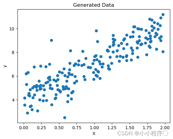
使用numpy随机生成数据

import numpy as np
import matplotlib.pyplot as plt

# 生成模拟数据
np.random.seed(42)
X = 2 * np.random.rand(200, 1)
y = 4 + 3 * X + np.random.randn(200, 1)

# 可视化数据
plt.scatter(X, y)
plt.xlabel('X')
plt.ylabel('y')
plt.title('Generated Data')
plt.show()

定义线性回归参数并实现梯度下降

对于线性拟合，其假设函数为：
$$h_{\theta }(x)={\theta }_{1}x+{\theta }_0$$
这其中的$\theta$是假设函数当中的参数。
也可以简化为：
$$h_{\theta }(x)={\theta }_{1}x$$

代价函数，在统计学上称为均方根误差函数。当假设函数中的系数$\theta$取不同的值时，$\frac{1}{2m}$倍假设函数预测值$h_{\theta }(x^{(i)})$和真实值$y^{(i)}$的差的平方的和之间的函数关系表示为代价函数$J$。
$$J({\theta }_0,{\theta }_1)=\frac{1}{2m}\sum _{i=1}^m(h_{\theta }(x^{(i)})-y^{(i)}{)}^2$$

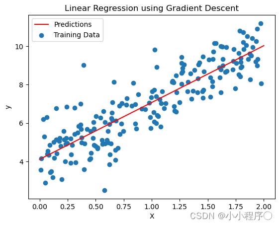
#x跟b
X_b=np.c_[np.ones((200,1)),X]

rate = 0.05 #学习率
iterations =1000 #迭代次数
m = 200 #样本数量

#参数theta
theta = np.random.randn(2,1)

#代价函数的梯度下降
for i in range(iterations):
    temp=1/m*X_b.T.dot(X_b.dot(theta)-y)
    theta=theta-rate*temp

print("参数是：",theta)

y=2.96103372*x+4.10512103

绘制预测完的图像

# 可视化结果
plt.plot(X_new, y_hat, "r-", label="Predictions")
plt.scatter(X, y, label="Training Data")
plt.xlabel('X')
plt.ylabel('y')
plt.legend()
plt.title('Linear Regression using Gradient Descent')
plt.show()

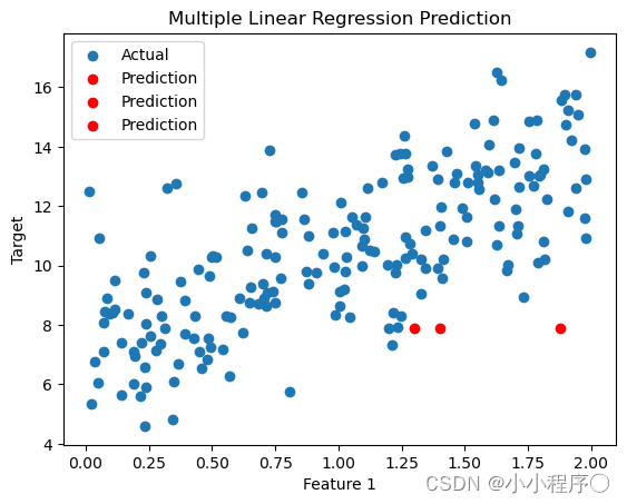
实现多元线性回归

多元线性回归的梯度下降算法：

$${\theta }_j:={\theta }_j-\alpha \frac{\partial J(\theta )}{\partial {\theta }_j}$$

对$\frac{\partial J(\theta )}{\partial {\theta }_j}$进行等价变形：

$${\theta }_j:={\theta }_j-\alpha \frac{1}{m}\sum _{i=1}^m(h_{\theta }(x^{(i)})-y^{(i)})x_j^i$$

#x跟b
X_b=np.c_[np.ones((200,1)),X]

rate = 0.05 #学习率
iterations =1000 #迭代次数
m = 200 #样本数量

#参数theta
theta = np.random.randn(4,1)

#梯度下降
for i in range(iterations):
    temp=1/m*X_b.T.dot(X_b.dot(theta)-y)
    theta=theta-rate*temp

print("参数是：",theta)


X_new=np.array([[1,1.3,3],[1.2,1.3,1.4],[1.1,1.2,1.88]])
X_b_new = np.c_[np.ones((3,1)),X_new]
y_hat = X_b_new.dot(theta)


# 可视化结果
plt.scatter(X[:, 0], y, label='Actual')
plt.scatter(X_new[0, 1], y_predict, color='red', label='Prediction')
plt.scatter(X_new[1, 2], y_predict, color='red', label='Prediction')
plt.scatter(X_new[2, 2], y_predict, color='red', label='Prediction')
plt.xlabel('Feature 1')
plt.ylabel('Target')
plt.legend()
plt.title('Multiple Linear Regression Prediction')
plt.show()