Pytorch深度学习案例5：运动鞋识别

一 前期准备

1.设置GPU 

import torch
import torch.nn as nn
import torchvision.transforms as transforms
import torchvision
from torchvision import transforms, datasets

import os,PIL,pathlib

device = torch.device("cuda" if torch.cuda.is_available() else "cpu")

device

 device(type='cpu')

2.导入数据 

import os,PIL,random,pathlib

data_dir = './shoes/'
data_dir = pathlib.Path(data_dir)

data_paths  = list(data_dir.glob('*'))
classeNames = [str(path).split("\\")[1] for path in data_paths]
classeNames

 熟悉一下这个案例的数据集结构：shoes文件夹下并没有直接的分类。如果是直接分类的话我们需要自行划分训练集和测试集，但此结构是shoes文件夹下有两个文件夹：train和test分别对应了训练集和测试集。每个文件夹下才是各种品牌运动鞋的分类。这也告诉我们当遇到自带的train和test文件如何处理

代码运行结果：['test', 'train'] 

• 第一步：使用pathlib.Path()函数将字符串类型的文件夹路径转换为pathlib.Path对象。
• 第二步：使用glob()方法获取data_dir路径下的所有文件路径，并以列表形式存储在data_paths中。
• 第三步：通过split()函数对data_paths中的每个文件路径执行分割操作，获得各个文件所属的类别名称，并存储在classeNames中
• 第四步：打印classeNames列表，显示每个文件所属的类别名称。

 

# 关于transforms.Compose的更多介绍可以参考：https://blog.csdn.net/qq_38251616/article/details/124878863
train_transforms = transforms.Compose([
    transforms.Resize([224, 224]),  # 将输入图片resize成统一尺寸
    # transforms.RandomHorizontalFlip(), # 随机水平翻转
    transforms.ToTensor(),          # 将PIL Image或numpy.ndarray转换为tensor，并归一化到[0,1]之间
    transforms.Normalize(           # 标准化处理-->转换为标准正太分布（高斯分布），使模型更容易收敛
        mean=[0.485, 0.456, 0.406], 
        std=[0.229, 0.224, 0.225])  # 其中 mean=[0.485,0.456,0.406]与std=[0.229,0.224,0.225] 从数据集中随机抽样计算得到的。
])

test_transform = transforms.Compose([
    transforms.Resize([224, 224]),  # 将输入图片resize成统一尺寸
    transforms.ToTensor(),          # 将PIL Image或numpy.ndarray转换为tensor，并归一化到[0,1]之间
    transforms.Normalize(           # 标准化处理-->转换为标准正太分布（高斯分布），使模型更容易收敛
        mean=[0.485, 0.456, 0.406], 
        std=[0.229, 0.224, 0.225])  # 其中 mean=[0.485,0.456,0.406]与std=[0.229,0.224,0.225] 从数据集中随机抽样计算得到的。
])

train_dataset = datasets.ImageFolder("./shoes/train/",transform=train_transforms)
test_dataset  = datasets.ImageFolder("./shoes/test/",transform=test_transform)
train_dataset.class_to_idx

{'adidas': 0, 'nike': 1} 

3.设置参数 

batch_size = 16

train_dl = torch.utils.data.DataLoader(train_dataset,
                                           batch_size=batch_size,
                                           shuffle=True,
                                           num_workers=1)
test_dl = torch.utils.data.DataLoader(test_dataset,
                                          batch_size=batch_size,
                                          shuffle=True,
                                          num_workers=1)
# 取一个批次查看数据格式
# 数据的shape为：[batch_size, channel, height, weight]
# 其中batch_size为自己设定，channel，height和weight分别是图片的通道数，高度和宽度。
imgs, labels = next(iter(train_dl))
imgs.shape

 Shape of X [N, C, H, W]:  torch.Size([8, 3, 224, 224])
 Shape of y:  torch.Size([8]) torch.int64

 4.展现图像数据

import matplotlib.pyplot as plt
from PIL import Image

# 指定图像文件夹路径
image_folder = './shoes/train/nike'

# 获取文件夹中的所有图像文件
image_files = [f for f in os.listdir(image_folder) if f.endswith((".jpg", ".png", ".jpeg"))]

# 创建Matplotlib图像
fig, axes = plt.subplots(3, 8, figsize=(16, 6))

# 使用列表推导式加载和显示图像
for ax, img_file in zip(axes.flat, image_files):
    img_path = os.path.join(image_folder, img_file)
    img = Image.open(img_path)
    ax.imshow(img)
    ax.axis('off')

# 显示图像
plt.tight_layout()
plt.show()

 

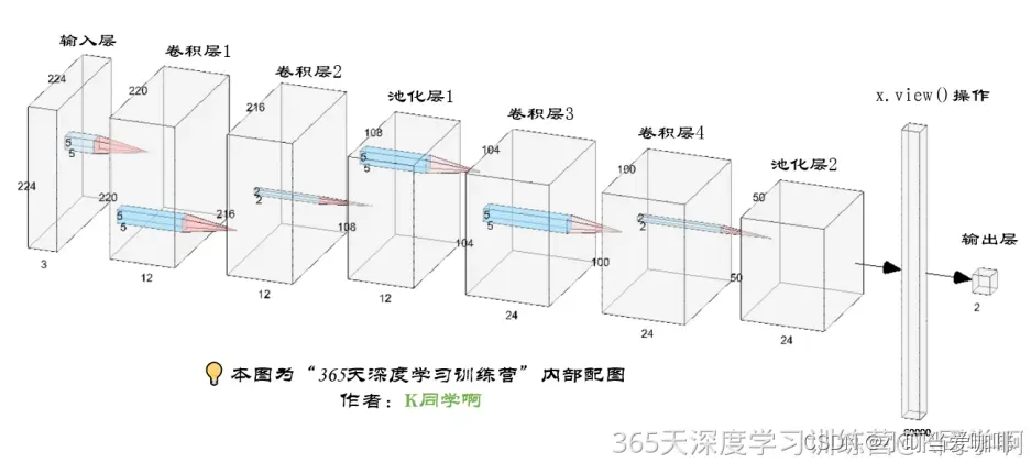
二 构建简单的CNN模型 

 

import torch.nn.functional as F

class Model(nn.Module):
    def __init__(self):
        super(Model, self).__init__()
        self.conv1=nn.Sequential(
            nn.Conv2d(3, 12, kernel_size=5, padding=0), # 12*220*220
            nn.BatchNorm2d(12),
            nn.ReLU())
        
        self.conv2=nn.Sequential(
            nn.Conv2d(12, 12, kernel_size=5, padding=0), # 12*216*216
            nn.BatchNorm2d(12),
            nn.ReLU())
        
        self.pool3=nn.Sequential(
            nn.MaxPool2d(2))                              # 12*108*108
        
        self.conv4=nn.Sequential(
            nn.Conv2d(12, 24, kernel_size=5, padding=0), # 24*104*104
            nn.BatchNorm2d(24),
            nn.ReLU())
        
        self.conv5=nn.Sequential(
            nn.Conv2d(24, 24, kernel_size=5, padding=0), # 24*100*100
            nn.BatchNorm2d(24),
            nn.ReLU())
        
        self.pool6=nn.Sequential(
            nn.MaxPool2d(2))                              # 24*50*50

        self.dropout = nn.Sequential(
            nn.Dropout(0.2))
        
        self.fc=nn.Sequential(
            nn.Linear(24*50*50, len(classeNames)))
        
    def forward(self, x):
        
        batch_size = x.size(0)
        x = self.conv1(x)  # 卷积-BN-激活
        x = self.conv2(x)  # 卷积-BN-激活
        x = self.pool3(x)  # 池化
        x = self.conv4(x)  # 卷积-BN-激活
        x = self.conv5(x)  # 卷积-BN-激活
        x = self.pool6(x)  # 池化
        x = self.dropout(x)
        x = x.view(batch_size, -1)  # flatten 变成全连接网络需要的输入 (batch, 24*50*50) ==> (batch, -1), -1 此处自动算出的是24*50*50
        x = self.fc(x)
       
        return x

device = "cuda" if torch.cuda.is_available() else "cpu"
print("Using {} device".format(device))

model = Model().to(device)
model

 

Using cuda device

Model(
  (conv1): Sequential(
    (0): Conv2d(3, 12, kernel_size=(5, 5), stride=(1, 1))
    (1): BatchNorm2d(12, eps=1e-05, momentum=0.1, affine=True, track_running_stats=True)
    (2): ReLU()
  )
  (conv2): Sequential(
    (0): Conv2d(12, 12, kernel_size=(5, 5), stride=(1, 1))
    (1): BatchNorm2d(12, eps=1e-05, momentum=0.1, affine=True, track_running_stats=True)
    (2): ReLU()
  )
  (pool3): Sequential(
    (0): MaxPool2d(kernel_size=2, stride=2, padding=0, dilation=1, ceil_mode=False)
  )
  (conv4): Sequential(
    (0): Conv2d(12, 24, kernel_size=(5, 5), stride=(1, 1))
    (1): BatchNorm2d(24, eps=1e-05, momentum=0.1, affine=True, track_running_stats=True)
    (2): ReLU()
  )
  (conv5): Sequential(
    (0): Conv2d(24, 24, kernel_size=(5, 5), stride=(1, 1))
    (1): BatchNorm2d(24, eps=1e-05, momentum=0.1, affine=True, track_running_stats=True)
    (2): ReLU()
  )
  (pool6): Sequential(
    (0): MaxPool2d(kernel_size=2, stride=2, padding=0, dilation=1, ceil_mode=False)
  )
  (dropout): Sequential(
    (0): Dropout(p=0.2, inplace=False)
  )
  (fc): Sequential(
    (0): Linear(in_features=60000, out_features=2, bias=True)
  )
)

三 训练模型

1.编写训练函数

# 训练循环
def train(dataloader, model, loss_fn, optimizer):
    size = len(dataloader.dataset)  # 训练集的大小
    num_batches = len(dataloader)   # 批次数目, (size/batch_size，向上取整)

    train_loss, train_acc = 0, 0  # 初始化训练损失和正确率
    
    for X, y in dataloader:  # 获取图片及其标签
        X, y = X.to(device), y.to(device)
        
        # 计算预测误差
        pred = model(X)          # 网络输出
        loss = loss_fn(pred, y)  # 计算网络输出和真实值之间的差距，targets为真实值，计算二者差值即为损失
        
        # 反向传播
        optimizer.zero_grad()  # grad属性归零
        loss.backward()        # 反向传播
        optimizer.step()       # 每一步自动更新
        
        # 记录acc与loss
        train_acc  += (pred.argmax(1) == y).type(torch.float).sum().item()
        train_loss += loss.item()
            
    train_acc  /= size
    train_loss /= num_batches

    return train_acc, train_loss

2.编写测试函数

def test (dataloader, model, loss_fn):
    size        = len(dataloader.dataset)  # 测试集的大小
    num_batches = len(dataloader)          # 批次数目, (size/batch_size，向上取整)
    test_loss, test_acc = 0, 0
    
    # 当不进行训练时，停止梯度更新，节省计算内存消耗
    with torch.no_grad():
        for imgs, target in dataloader:
            imgs, target = imgs.to(device), target.to(device)
            
            # 计算loss
            target_pred = model(imgs)
            loss        = loss_fn(target_pred, target)
            
            test_loss += loss.item()
            test_acc  += (target_pred.argmax(1) == target).type(torch.float).sum().item()

    test_acc  /= size
    test_loss /= num_batches

    return test_acc, test_loss

 3.设置动态学习率

# 调用官方动态学习率接口时使用
learn_rate = 1e-4 # 初始学习率
lambda1 = lambda epoch: (0.92 ** (epoch // 2))
optimizer = torch.optim.SGD(model.parameters(), lr=learn_rate)
scheduler = torch.optim.lr_scheduler.LambdaLR(optimizer, lr_lambda=lambda1) #选定调整方法

 4.正式训练

loss_fn    = nn.CrossEntropyLoss() # 创建损失函数
epochs     = 40

train_loss = []
train_acc  = []
test_loss  = []
test_acc   = []

for epoch in range(epochs):    
    model.train()
    epoch_train_acc, epoch_train_loss = train(train_dl, model, loss_fn, optimizer)
    # scheduler.step() # 更新学习率（调用官方动态学习率接口时使用）
    
    model.eval()
    epoch_test_acc, epoch_test_loss = test(test_dl, model, loss_fn)
    
    train_acc.append(epoch_train_acc)
    train_loss.append(epoch_train_loss)
    test_acc.append(epoch_test_acc)
    test_loss.append(epoch_test_loss)
    
    # 获取当前的学习率
    lr = optimizer.state_dict()['param_groups'][0]['lr']
    
    template = ('Epoch:{:2d}, Train_acc:{:.1f}%, Train_loss:{:.3f}, Test_acc:{:.1f}%, Test_loss:{:.3f}, Lr:{:.2E}')
    print(template.format(epoch+1, epoch_train_acc*100, epoch_train_loss, 
                          epoch_test_acc*100, epoch_test_loss, lr))
print('Done')

 

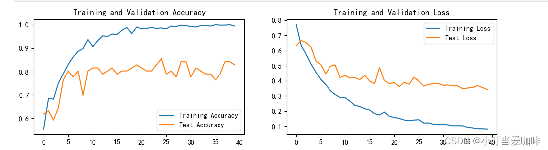
Epoch: 1, Train_acc:55.4%, Train_loss:0.770, Test_acc:61.8%, Test_loss:0.632, Lr:1.00E-04
Epoch: 2, Train_acc:68.5%, Train_loss:0.634, Test_acc:63.2%, Test_loss:0.666, Lr:1.00E-04
Epoch: 3, Train_acc:68.1%, Train_loss:0.577, Test_acc:59.2%, Test_loss:0.653, Lr:1.00E-04
Epoch: 4, Train_acc:74.9%, Train_loss:0.512, Test_acc:64.5%, Test_loss:0.623, Lr:1.00E-04
Epoch: 5, Train_acc:79.1%, Train_loss:0.458, Test_acc:76.3%, Test_loss:0.533, Lr:1.00E-04
Epoch: 6, Train_acc:83.1%, Train_loss:0.409, Test_acc:80.3%, Test_loss:0.508, Lr:1.00E-04
Epoch: 7, Train_acc:86.3%, Train_loss:0.375, Test_acc:77.6%, Test_loss:0.446, Lr:1.00E-04
Epoch: 8, Train_acc:88.6%, Train_loss:0.334, Test_acc:80.3%, Test_loss:0.497, Lr:1.00E-04
Epoch: 9, Train_acc:89.8%, Train_loss:0.309, Test_acc:69.7%, Test_loss:0.506, Lr:1.00E-04
Epoch:10, Train_acc:93.6%, Train_loss:0.289, Test_acc:80.3%, Test_loss:0.421, Lr:1.00E-04
Epoch:11, Train_acc:90.6%, Train_loss:0.289, Test_acc:81.6%, Test_loss:0.436, Lr:1.00E-04
Epoch:12, Train_acc:93.2%, Train_loss:0.265, Test_acc:81.6%, Test_loss:0.418, Lr:1.00E-04
Epoch:13, Train_acc:95.2%, Train_loss:0.238, Test_acc:78.9%, Test_loss:0.420, Lr:1.00E-04
Epoch:14, Train_acc:95.0%, Train_loss:0.230, Test_acc:80.3%, Test_loss:0.407, Lr:1.00E-04
Epoch:15, Train_acc:96.0%, Train_loss:0.216, Test_acc:81.6%, Test_loss:0.435, Lr:1.00E-04
Epoch:16, Train_acc:95.8%, Train_loss:0.208, Test_acc:78.9%, Test_loss:0.398, Lr:1.00E-04
Epoch:17, Train_acc:97.6%, Train_loss:0.183, Test_acc:80.3%, Test_loss:0.381, Lr:1.00E-04
Epoch:18, Train_acc:98.8%, Train_loss:0.175, Test_acc:80.3%, Test_loss:0.489, Lr:1.00E-04
Epoch:19, Train_acc:96.2%, Train_loss:0.194, Test_acc:81.6%, Test_loss:0.400, Lr:1.00E-04
Epoch:20, Train_acc:99.0%, Train_loss:0.166, Test_acc:82.9%, Test_loss:0.381, Lr:1.00E-04
Epoch:21, Train_acc:98.2%, Train_loss:0.158, Test_acc:81.6%, Test_loss:0.388, Lr:1.00E-04
Epoch:22, Train_acc:98.4%, Train_loss:0.152, Test_acc:80.3%, Test_loss:0.361, Lr:1.00E-04
Epoch:23, Train_acc:98.8%, Train_loss:0.141, Test_acc:80.3%, Test_loss:0.389, Lr:1.00E-04
Epoch:24, Train_acc:98.4%, Train_loss:0.136, Test_acc:82.9%, Test_loss:0.376, Lr:1.00E-04
Epoch:25, Train_acc:98.6%, Train_loss:0.141, Test_acc:85.5%, Test_loss:0.424, Lr:1.00E-04
Epoch:26, Train_acc:98.2%, Train_loss:0.143, Test_acc:78.9%, Test_loss:0.397, Lr:1.00E-04
Epoch:27, Train_acc:99.4%, Train_loss:0.121, Test_acc:80.3%, Test_loss:0.365, Lr:1.00E-04
Epoch:28, Train_acc:99.2%, Train_loss:0.122, Test_acc:77.6%, Test_loss:0.377, Lr:1.00E-04
Epoch:29, Train_acc:99.8%, Train_loss:0.113, Test_acc:84.2%, Test_loss:0.379, Lr:1.00E-04
Epoch:30, Train_acc:99.6%, Train_loss:0.110, Test_acc:84.2%, Test_loss:0.382, Lr:1.00E-04
Epoch:31, Train_acc:99.2%, Train_loss:0.111, Test_acc:77.6%, Test_loss:0.370, Lr:1.00E-04
Epoch:32, Train_acc:99.0%, Train_loss:0.109, Test_acc:81.6%, Test_loss:0.372, Lr:1.00E-04
Epoch:33, Train_acc:99.6%, Train_loss:0.103, Test_acc:80.3%, Test_loss:0.366, Lr:1.00E-04
Epoch:34, Train_acc:99.6%, Train_loss:0.104, Test_acc:78.9%, Test_loss:0.366, Lr:1.00E-04
Epoch:35, Train_acc:99.4%, Train_loss:0.103, Test_acc:78.9%, Test_loss:0.346, Lr:1.00E-04
Epoch:36, Train_acc:100.0%, Train_loss:0.093, Test_acc:76.3%, Test_loss:0.352, Lr:1.00E-04
Epoch:37, Train_acc:99.8%, Train_loss:0.090, Test_acc:78.9%, Test_loss:0.355, Lr:1.00E-04
Epoch:38, Train_acc:99.8%, Train_loss:0.084, Test_acc:84.2%, Test_loss:0.367, Lr:1.00E-04
Epoch:39, Train_acc:100.0%, Train_loss:0.084, Test_acc:84.2%, Test_loss:0.355, Lr:1.00E-04
Epoch:40, Train_acc:99.4%, Train_loss:0.082, Test_acc:82.9%, Test_loss:0.341, Lr:1.00E-04
Done

四 结果可视化

1.loss和Accuary图 

 

2.指定图片预测 

⭐torch.squeeze()详解
对数据的维度进行压缩，去掉维数为1的的维度

函数原型：
torch.squeeze(input, dim=None, *, out=None)

关键参数说明：
● input (Tensor)：输入Tensor
● dim (int, optional)：如果给定，输入将只在这个维度上被压缩

from PIL import Image 

classes = list(train_dataset.class_to_idx)

def predict_one_image(image_path, model, transform, classes):
    
    test_img = Image.open(image_path).convert('RGB')
    # plt.imshow(test_img)  # 展示预测的图片

    test_img = transform(test_img)
    img = test_img.to(device).unsqueeze(0)
    
    model.eval()
    output = model(img)

    _,pred = torch.max(output,1)
    pred_class = classes[pred]
    print(f'预测结果是：{pred_class}')

# 预测训练集中的某张照片
predict_one_image(image_path='./shoes/test/adidas/1.jpg', 
                  model=model, 
                  transform=train_transforms, 
                  classes=classes)

预测结果是：adidas

五 保存模型 

# 模型保存
PATH = './model.pth'  # 保存的参数文件名
torch.save(model.state_dict(), PATH)

# 将参数加载到model当中
model.load_state_dict(torch.load(PATH, map_location=device))