


目录
SHAP (SHapley Additive exPlanations) 可视化笔记
2. UCI Machine Learning Repository
2. COCO (Common Objects in Context)
2. SQuAD (Stanford Question Answering Dataset)
SHAP (SHapley Additive exPlanations) 可视化笔记
SHAP 是一种基于博弈论的解释机器学习模型预测的方法,可以提供直观的特征重要性分析和单个预测的解释。
一、SHAP 基础概念
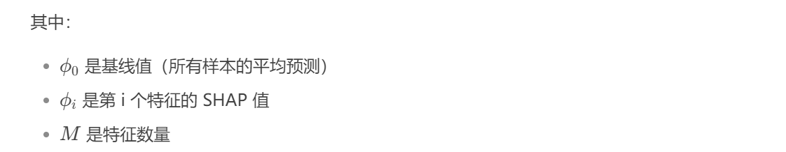
1.1 SHAP 值核心思想
-
基于博弈论的 Shapley 值
-
量化每个特征对模型预测的贡献度
-
满足可加性:所有特征的 SHAP 值之和等于预测值与平均预测的差值
1.2 SHAP 值的数学表达
对于单个样本的预测:

二、SHAP 可视化类型
2.1 全局特征重要性
2.1.1 条形图
import shap

# 创建解释器
explainer = shap.Explainer(model)
shap_values = explainer(X)

# 全局特征重要性
shap.plots.bar(shap_values)解读:
-
按平均绝对 SHAP 值降序排列
-
显示各特征对模型输出的总体影响
2.1.2 蜂群图 (Beeswarm Plot)
shap.plots.beeswarm(shap_values)特点:
-
展示特征值与 SHAP 值的关系
-
颜色表示特征值高低
-
点密度反映样本分布
2.2 局部解释
2.2.1 单个预测解释
# 解释单个样本
shap.plots.waterfall(shap_values[0]) # 第一个样本解读:
-
显示从基线值到预测值的"流动"
-
每个特征推动预测增加或减少
2.2.2 力图 (Force Plot)
shap.plots.force(shap_values[0])特点:
-
直观显示各特征对当前预测的贡献
-
红色表示正向推动,蓝色表示负向推动
2.3 交互作用可视化
2.3.1 依赖图
shap.plots.scatter(shap_values[:, "feature_name"])解读:
-
显示某个特征的 SHAP 值如何随特征值变化
-
可发现非线性关系和阈值效应
2.3.2 交互作用图
shap.plots.scatter(shap_values[:, "feature1"], color=shap_values[:, "feature2"])解读:
-
显示两个特征的交互作用
-
颜色表示第二个特征的值
三、SHAP 高级应用
3.1 模型比较
# 比较两个模型的 SHAP 值
explainer1 = shap.Explainer(model1)
explainer2 = shap.Explainer(model2)
shap_values1 = explainer1(X)
shap_values2 = explainer2(X)

shap.plots.scatter(shap_values1[:, "feature"], color=shap_values2[:, "feature"])
3.2 聚类分析
# 基于 SHAP 值聚类
clustering = shap.utils.hclust(X, shap_values)
shap.plots.bar(shap_values, clustering=clustering)
3.3 文本和图像解释
# 文本模型解释
explainer = shap.Explainer(text_model)
shap_values = explainer([text_sample])
shap.plots.text(shap_values)

# 图像模型解释
explainer = shap.Explainer(image_model)
shap_values = explainer([image_array])
shap.image_plot(shap_values, [image_array])
四、SHAP 使用技巧
4.1 加速计算
# 使用近似方法
explainer = shap.Explainer(model, algorithm="permutation")

# 对样本子集计算
shap_values = explainer(X[:100])  # 只计算前100个样本
4.2 处理分类特征
# 使用独热编码
X_encoded = pd.get_dummies(X, columns=["categorical_feature"])

# 或者使用 Partition 解释器
explainer = shap.PartitionExplainer(model, X)
4.3 自定义可视化
# 修改颜色和样式
shap.plots.beeswarm(shap_values, color=plt.get_cmap("coolwarm"))
五、SHAP 可视化解读指南
| 可视化类型 | 适用场景 | 关键解读点 |
|---|---|---|
| 条形图 | 全局特征重要性 | 特征对模型输出的总体影响排序 |
| 蜂群图 | 特征影响分布 | 特征值与 SHAP 值的关系、数据分布 |
| 力图 | 单个预测解释 | 各特征对特定预测的具体贡献 |
| 依赖图 | 特征效应分析 | 特征与预测的非线性关系 |
| 交互图 | 特征交互作用 | 两个特征如何共同影响预测 |
六、完整示例代码
import shap
import pandas as pd
from sklearn.ensemble import RandomForestClassifier
import matplotlib.pyplot as plt

# 1. 准备数据和模型
# 假设 X_train, y_train 已经准备好
model = RandomForestClassifier().fit(X_train, y_train)

# 2. 创建 SHAP 解释器
explainer = shap.Explainer(model)
shap_values = explainer(X_train)

# 3. 全局解释
plt.figure(figsize=(10, 6))
shap.plots.bar(shap_values, show=False)
plt.title("Global Feature Importance")
plt.tight_layout()
plt.show()

# 4. 蜂群图
plt.figure(figsize=(10, 6))
shap.plots.beeswarm(shap_values, show=False)
plt.title("Feature Effects")
plt.tight_layout()
plt.show()

# 5. 单个样本解释
sample_idx = 0  # 解释第一个样本
shap.plots.waterfall(shap_values[sample_idx])

# 6. 特征依赖分析
feature_name = "age"  # 分析age特征
shap.plots.scatter(shap_values[:, feature_name])
七、注意事项
-
计算资源:
-
SHAP 计算可能很耗时,特别是对大型数据集
-
树模型可以使用 TreeSHAP 加速,其他模型考虑使用 KernelSHAP 或抽样
-
-
模型支持:
-
TreeSHAP 适用于树模型(随机森林、XGBoost 等)
-
KernelSHAP 适用于任何模型,但计算更慢
-
-
解释一致性:
-
SHAP 值会因随机种子不同而略有变化
-
对重要结论建议多次运行验证
-
-
特征相关性:
-
当特征高度相关时,SHAP 解释可能不稳定
-
考虑使用 SHAP 交互值或聚类分析
-
SHAP 提供了强大的模型解释能力,帮助理解模型行为、验证特征重要性,并识别潜在的偏差问题。正确解读 SHAP 可视化结果对于模型调试和业务解释至关重要。
开源数据集平台大全
一、综合型数据集平台
1. Kaggle Datasets
-
网址: Find Open Datasets and Machine Learning Projects | Kaggle
-
特点:
-
超过5万个公开数据集
-
涵盖计算机视觉、自然语言处理、时间序列等多个领域
-
配套提供Notebook环境和社区讨论
-
2. UCI Machine Learning Repository
-
特点:
-
最古老的机器学习数据集库之一(1987年创建)
-
包含400+个经典数据集
-
每个数据集都有详细的元数据描述
-
3. Google Dataset Search
-
特点:
-
Google开发的跨平台数据集搜索引擎
-
索引来自各领域的2500万+数据集
-
支持按许可证类型、更新时间等筛选
-
二、计算机视觉数据集
1. ImageNet
-
网址: ImageNet
-
特点:
-
1400万张标注图像,2万多个类别
-
年度ILSVRC比赛的基础数据集
-
需要注册申请访问权限
-
2. COCO (Common Objects in Context)
-
特点:
-
33万张图像,80个物体类别
-
包含目标检测、分割、关键点标注
-
提供标准的评估指标
-
3. Open Images Dataset
-
网址: Open Images V7
-
特点:
-
Google提供的900万张图像数据集
-
包含图像级标签、边界框和分割掩码
-
6000个物体类别
-
三、自然语言处理数据集
1. Hugging Face Datasets
-
特点:
-
提供1000+个NLP数据集
-
统一的数据加载API
-
支持流式加载大数据集
-
2. SQuAD (Stanford Question Answering Dataset)
-
特点:
-
阅读理解任务的标准基准
-
包含10万+问答对
-
有1.0和2.0两个版本
-
3. GLUE Benchmark
-
网址: GLUE Benchmark
-
特点:
-
9个不同的NLP任务数据集
-
用于评估模型的语言理解能力
-
已被SuperGLUE基准取代
-
四、科学和学术数据集
1. Figshare
-
特点:
-
学术研究成果的数据集平台
-
支持各种格式的数据上传
-
提供DOI便于引用
-
2. Dryad
-
特点:
-
专注于科学出版物的配套数据
-
强制要求CC0许可证(完全开放)
-
特别适合生命科学领域
-
3. Zenodo
-
网址: Zenodo
-
特点:
-
由CERN运营的开放研究数据平台
-
支持50GB以内的数据集上传
-
为每个数据集分配DOI
-
五、政府和公共数据
1. World Bank Open Data
-
特点:
-
全球发展指标的权威来源
-
包含3000+个经济和社会指标
-
支持多种格式下载
-
2. NASA Open Data
-
特点:
-
地球科学、航空航天等领域数据集
-
包含卫星图像、气候数据等
-
部分数据集实时更新
-
3. EU Open Data Portal
-
特点:
-
欧盟机构发布的开放数据
-
涵盖经济、就业、环境等领域
-
多语言支持
-
六、特定领域数据集
1. 医学和生物信息学
-
TCGA (癌症基因组图谱): The Cancer Genome Atlas Program (TCGA) - NCI
-
UK Biobank: UK Biobank - UK Biobank
-
MIMIC-III: MIMIC
2. 地理空间数据
-
OpenStreetMap: https://www.openstreetmap.org/
-
USGS Earth Explorer: https://earthexplorer.usgs.gov/
-
Sentinel Hub: Sentinel Hub
3. 金融和经济
-
Quandl: Financial, Economic and Alternative Data | Nasdaq Data Link
-
Yahoo Finance: https://finance.yahoo.com/
-
FRED Economic Data: Federal Reserve Economic Data | FRED | St. Louis Fed
完整示例(我的专业相关:WiFi 数据集,来自kaggleWi-Fi Indoor Localization Dataset (WILD-v2) | Kaggle)
步骤一:数据预处理
import pandas as pd
import pandas as pd    #用于数据处理和分析,可处理表格数据。
import numpy as np     #用于数值计算,提供了高效的数组操作。
import matplotlib.pyplot as plt    #用于绘制各种类型的图表
import seaborn as sns   #基于matplotlib的高级绘图库,能绘制更美观的统计图形。
import warnings
warnings.filterwarnings("ignore")

 # 设置中文字体(解决中文显示问题)
plt.rcParams['font.sans-serif'] = ['SimHei']  # Windows系统常用黑体字体
plt.rcParams['axes.unicode_minus'] = False    # 正常显示负号
data = pd.read_csv('sample_solution.csv')    #读取数据
# Environment 1-0映射
Environment_mapping = {
    '4floor':0,
    '5floor':1
}
data['Environment'] = data['Environment'].map(Environment_mapping)
data.rename(columns={'Environment4': 'Environment5'}, inplace=True) # 重命名列
continuous_features = data.select_dtypes(include=['int64', 'float64']).columns.tolist()  #把筛选出来的列名转换成列表
data.head()

# 最开始也说了 很多调参函数自带交叉验证,甚至是必选的参数,你如果想要不交叉反而实现起来会麻烦很多
# 所以这里我们还是只划分一次数据集
from sklearn.model_selection import train_test_split
X = data.drop(['Environment'], axis=1)  # 特征,axis=1表示按列删除
y = data['Environment'] # 标签
# 按照8:2划分训练集和测试集
X_train, X_test, y_train, y_test = train_test_split(X, y, test_size=0.2, random_state=42)  # 80%训练集,20%测试集
步骤二 超参数优化
基础超参数优化
from sklearn.ensemble import RandomForestClassifier #随机森林分类器

from sklearn.metrics import accuracy_score, precision_score, recall_score, f1_score # 用于评估分类器性能的指标
from sklearn.metrics import classification_report, confusion_matrix #用于生成分类报告和混淆矩阵
import warnings #用于忽略警告信息
warnings.filterwarnings("ignore") # 忽略所有警告信息
# --- 1. 默认参数的随机森林 ---
# 评估基准模型,这里确实不需要验证集
print("--- 1. 默认参数随机森林 (训练集 -> 测试集) ---")
import time # 这里介绍一个新的库,time库,主要用于时间相关的操作,因为调参需要很长时间,记录下会帮助后人知道大概的时长
start_time = time.time() # 记录开始时间
rf_model = RandomForestClassifier(random_state=42)
rf_model.fit(X_train, y_train) # 在训练集上训练
rf_pred = rf_model.predict(X_test) # 在测试集上预测
end_time = time.time() # 记录结束时间

print(f"训练与预测耗时: {end_time - start_time:.4f} 秒")
print("\n默认随机森林 在测试集上的分类报告:")
print(classification_report(y_test, rf_pred))
print("默认随机森林 在测试集上的混淆矩阵:")
print(confusion_matrix(y_test, rf_pred))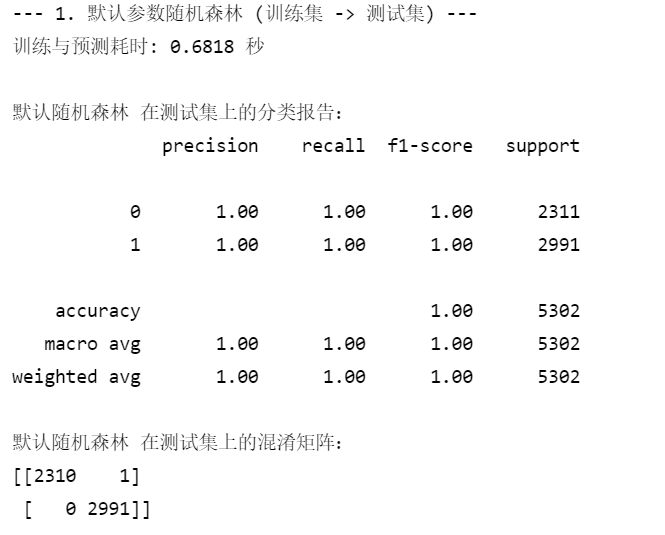
退火算法对比性能
import random
# --- 2. 模拟退火算法优化随机森林 ---
print("\n--- 2. 模拟退火算法优化随机森林 (训练集 -> 测试集) ---")


# 定义适应度函数
def fitness_function(params):
    n_estimators, max_depth, min_samples_split, min_samples_leaf = params
    model = RandomForestClassifier(n_estimators=int(n_estimators),
                                   max_depth=int(max_depth),
                                   min_samples_split=int(min_samples_split),
                                   min_samples_leaf=int(min_samples_leaf),
                                   random_state=42)
    model.fit(X_train, y_train)
    y_pred = model.predict(X_test)
    accuracy = accuracy_score(y_test, y_pred)
    return accuracy


# 模拟退火算法实现
def simulated_annealing(initial_solution, bounds, initial_temp, final_temp, alpha):
    current_solution = initial_solution
    current_fitness = fitness_function(current_solution)
    best_solution = current_solution
    best_fitness = current_fitness
    temp = initial_temp

    while temp > final_temp:
        # 生成邻域解
        neighbor_solution = []
        for i in range(len(current_solution)):
            new_val = current_solution[i] + random.uniform(-1, 1) * (bounds[i][1] - bounds[i][0]) * 0.1
            new_val = max(bounds[i][0], min(bounds[i][1], new_val))
            neighbor_solution.append(new_val)

        neighbor_fitness = fitness_function(neighbor_solution)
        delta_fitness = neighbor_fitness - current_fitness

        if delta_fitness > 0 or random.random() < np.exp(delta_fitness / temp):
            current_solution = neighbor_solution
            current_fitness = neighbor_fitness

        if current_fitness > best_fitness:
            best_solution = current_solution
            best_fitness = current_fitness

        temp *= alpha

    return best_solution, best_fitness


# 超参数范围
bounds = [(50, 200), (10, 30), (2, 10), (1, 4)]  # n_estimators, max_depth, min_samples_split, min_samples_leaf

# 模拟退火算法参数
initial_temp = 100 # 初始温度
final_temp = 0.1 # 终止温度
alpha = 0.95 # 温度衰减系数

# 初始化初始解
initial_solution = [random.uniform(bounds[i][0], bounds[i][1]) for i in range(len(bounds))]

start_time = time.time()
best_params, best_fitness = simulated_annealing(initial_solution, bounds, initial_temp, final_temp, alpha)
end_time = time.time()

print(f"模拟退火算法优化耗时: {end_time - start_time:.4f} 秒")
print("最佳参数: ", {
    'n_estimators': int(best_params[0]),
    'max_depth': int(best_params[1]),
    'min_samples_split': int(best_params[2]),
    'min_samples_leaf': int(best_params[3])
})

# 使用最佳参数的模型进行预测
best_model = RandomForestClassifier(n_estimators=int(best_params[0]),
                                    max_depth=int(best_params[1]),
                                    min_samples_split=int(best_params[2]),
                                    min_samples_leaf=int(best_params[3]),
                                    random_state=42)
best_model.fit(X_train, y_train)
best_pred = best_model.predict(X_test)

print("\n模拟退火算法优化后的随机森林 在测试集上的分类报告:")
print(classification_report(y_test, best_pred))
print("模拟退火算法优化后的随机森林 在测试集上的混淆矩阵:")
print(confusion_matrix(y_test, best_pred))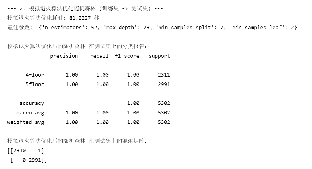
步骤三:shap库绘制图形
import lightgbm as lgb
from sklearn.model_selection import train_test_split, StratifiedKFold
from sklearn.metrics import roc_auc_score
from imblearn.over_sampling import SMOTE

# 划分训练集和测试集
X_train, X_test, y_train, y_test = train_test_split(X, y, test_size=0.2, random_state=42)

# 定义SMOTE对象
smote = SMOTE(random_state=42)

# 定义LightGBM模型
lgb_model = lgb.LGBMClassifier(random_state=42)

# 定义交叉验证对象
kfold = StratifiedKFold(n_splits=5, shuffle=True, random_state=42)

# 存储每次交叉验证的AUC分数
cv_scores = []

# 进行交叉验证
for train_index, val_index in kfold.split(X_train, y_train):
    X_train_fold, X_val_fold = X_train.iloc[train_index], X_train.iloc[val_index]
    y_train_fold, y_val_fold = y_train.iloc[train_index], y_train.iloc[val_index]

    # 对训练集进行过采样
    X_train_resampled, y_train_resampled = smote.fit_resample(X_train_fold, y_train_fold)

    # 训练模型
    lgb_model.fit(X_train_resampled, y_train_resampled)

    # 在验证集上进行预测
    y_val_pred_proba = lgb_model.predict_proba(X_val_fold)[:, 1]

    # 计算验证集的AUC分数
    val_auc = roc_auc_score(y_val_fold, y_val_pred_proba)
    cv_scores.append(val_auc)

# 输出交叉验证的平均AUC分数
print('交叉验证平均AUC: ', sum(cv_scores) / len(cv_scores)) 
import shap
explainer = shap.Explainer(lgb_model)
shap_values2 = explainer(X_test)
# 输出shap.Explanation对象
shap_values = explainer.shap_values(X) # 输出numpy.array数组
import matplotlib.pyplot as plt
shap.plots.bar(shap_values2)
plt.show() #plots.bar中的shap_values是 shap.Explanation对象
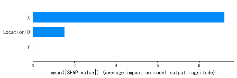
shap.summary_plot(shap_values,X,
plot_type="bar")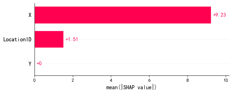
shap.plots.bar(shap_values2[1], show_data=True)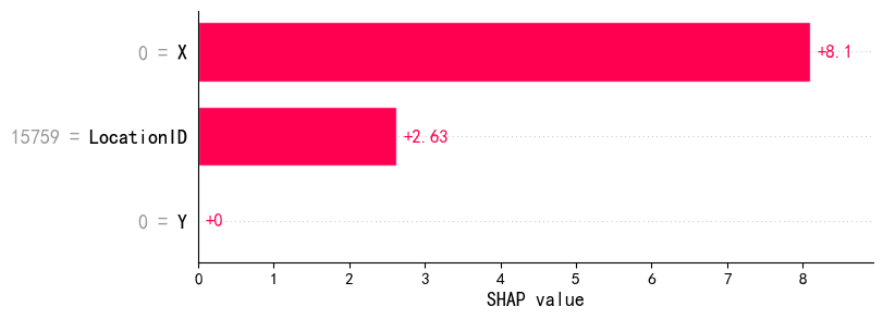
# 绘制队列条形图
# 选择一个特征进行分组,这里以 LocationID 为例,当 LocationID 大于中位数时标记为 High Income,否则标记为 Low Income
import numpy as np
median_income = np.median(X_test['LocationID'])
income_group = ["High Income" if X_test['LocationID'].iloc[i] > median_income
                else "Low Income" for i in range(X_test.shape[0])]

# 按分组计算绝对值的均值并绘制条形图
shap.plots.bar(shap_values2.cohorts(income_group).abs.mean(0))# 此处必须使用shap.Explanation 对象的函数。 shap.Explanation 对象才包含 cohorts 方法,而 numpy.ndarray 不包含。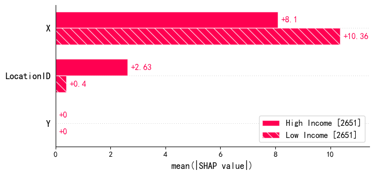
from sklearn.tree import DecisionTreeRegressor
# 设置队列数量
N = 3

cohorts = shap.Explainer(lgb_model)(X_test).cohorts(N)
# 绘制分组后的 SHAP 条形图
shap.plots.bar(cohorts.abs.mean(0))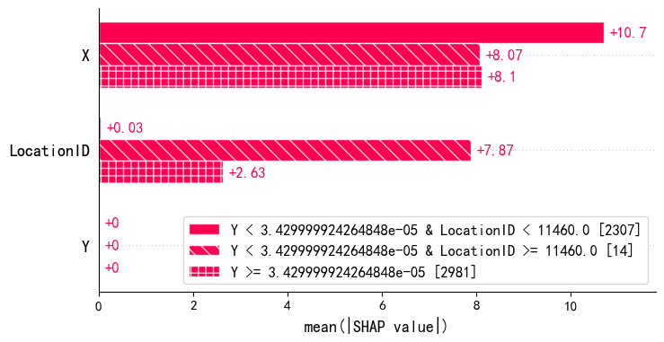
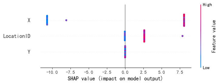
shap.summary_plot(shap_values, X)
shap.plots.beeswarm(shap_values2,
                    order=shap_values2.abs.max(0)) #默认是按照平均值排序,但此处按最大绝对值排序。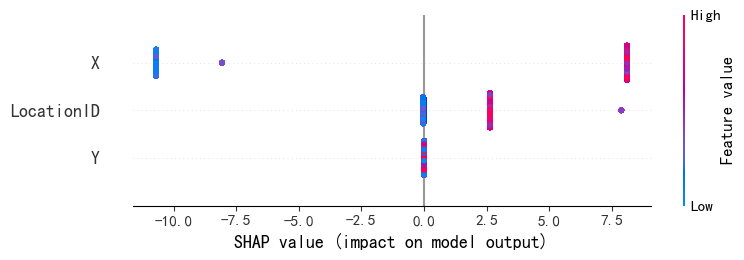
import shap
explainer = shap.Explainer(lgb_model)
shap_values2 = explainer(X_test)
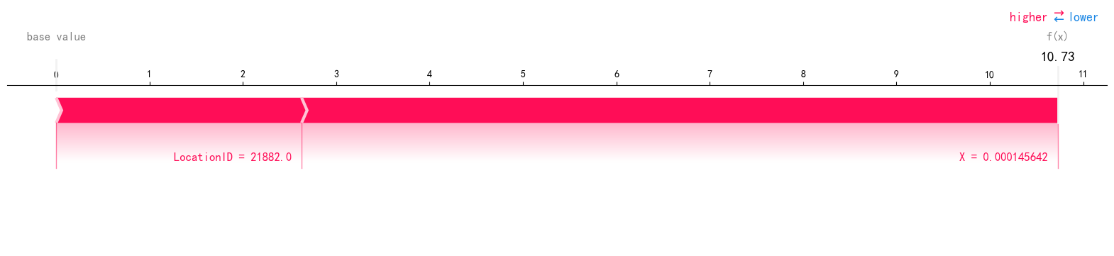
# 选择要分析的样本索引,这里以第一个样本为例
sample_index = 0
# 绘制单个样本的 force plot
shap.force_plot(explainer.expected_value, shap_values2[sample_index].values, X_test.iloc[sample_index], matplotlib=True)
import shap
# 创建解释器
explainer = shap.Explainer(lgb_model)
# 计算 SHAP 值
shap_values2 = explainer(X_test)

# 获取预期值,根据模型类型不同,预期值可能在不同位置
if isinstance(shap_values2, list):
    expected_value = explainer.expected_value[1]
    shap_values = shap_values2[1]
else:
    expected_value = explainer.expected_value
    shap_values = shap_values2.values

# 选择前 20 个样本进行可视化,可根据需求调整
sample_indices = range(20)
selected_shap_values = shap_values[sample_indices]
selected_features = X_test.iloc[sample_indices]

# 绘制 Decision plot
shap.decision_plot(expected_value, selected_shap_values, selected_features)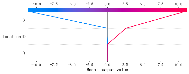
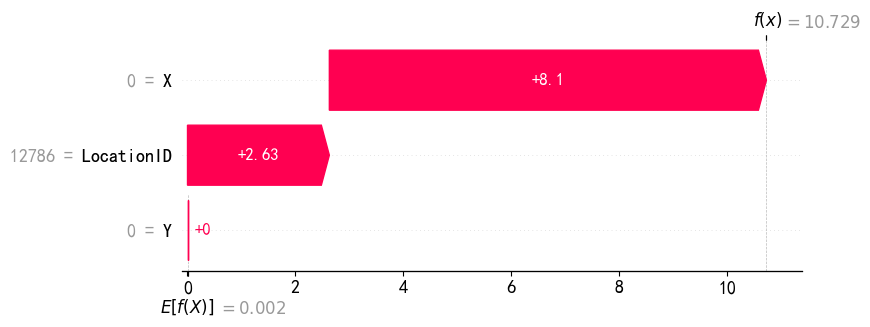
shap.plots.waterfall(shap_values2[5])


 299
299

 被折叠的 条评论
为什么被折叠?
被折叠的 条评论
为什么被折叠?
 到【灌水乐园】发言


