


一、简单的模型(类似“hello world")
mnist:其中有六万张训练图片,以及一万张测试图片
from tensorflow.keras.datasets import mnist
(train_images, train_labels), (test_images, test_labels) = mnist.load_data()

train_images.shape

len(train_labels)

train_labels

test_images.shape

len(test_labels)


test_labels

from tensorflow import keras
from tensorflow.keras import layers
model = keras.Sequential([
    layers.Dense(512, activation="relu"),
    layers.Dense(10, activation="softmax")
])

model.compile(optimizer="rmsprop",
              loss="sparse_categorical_crossentropy",
              metrics=["accuracy"])

train_images = train_images.reshape((60000, 28 * 28))
train_images = train_images.astype("float32") / 255
test_images = test_images.reshape((10000, 28 * 28))
test_images = test_images.astype("float32") / 255

model.fit(train_images, train_labels, epochs=5, batch_size=128)
#epochs 表示整个模型执行五次
model.compile()方法用于在配置训练方法时,告知训练时用的优化器、损失函数和准确率评测标准
model.compile(optimizer = 优化器,
loss = 损失函数,
metrics = ["准确率”])
其中:
optimizer可以是字符串形式给出的优化器名字,也可以是函数形式,使用函数形式可以设置学习率、动量和超参数
例如:“sgd” 或者 tf.optimizers.SGD(lr = 学习率,
decay = 学习率衰减率,
momentum = 动量参数)
“adagrad" 或者 tf.keras.optimizers.Adagrad(lr = 学习率,
decay = 学习率衰减率)
”adadelta" 或者 tf.keras.optimizers.Adadelta(lr = 学习率,
decay = 学习率衰减率)
“adam" 或者 tf.keras.optimizers.Adam(lr = 学习率,
decay = 学习率衰减率)
loss可以是字符串形式给出的损失函数的名字,也可以是函数形式
例如:”mse" 或者 tf.keras.losses.MeanSquaredError()
"sparse_categorical_crossentropy" 或者 tf.keras.losses.SparseCatagoricalCrossentropy(from_logits = False)
损失函数经常需要使用softmax函数来将输出转化为概率分布的形式,在这里from_logits代表是否将输出转为概率分布的形式,为False时表示转换为概率分布,为True时表示不转换,直接输出
Metrics标注网络评价指标
例如:
"accuracy" : y_ 和 y 都是数值,如y_ = [1] y = [1] #y_为真实值,y为预测值
“sparse_accuracy":y_和y都是以独热码 和概率分布表示,如y_ = [0, 1, 0], y = [0.256, 0.695, 0.048]
"sparse_categorical_accuracy" :y_是以数值形式给出,y是以 独热码给出,如y_ = [1], y = [0.256 0.695, 0.048]
————————————————
版权声明:本文为CSDN博主「yunfeather」的原创文章,遵循CC 4.0 BY-SA版权协议,转载请附上原文出处链接及本声明。
原文链接:https://blog.csdn.net/yunfeather/article/details/106461754
model.fit(train_images, train_labels, epochs=5, batch_size=128)
执行该函数相当于开始估计参数
用之前定义的network调用fit函数执行循环训练,在fit中的参数,train_image和train_labels是训练要使用的图片数据和标签,epochs是指训练多少次,batch_size是指一次训练多少个数据。
二、Data representations for neural networks 维度
在深度学习里,Tensor实际上就是一个多维数组(multidimensional array)。
而Tensor的目的是能够创造更高维度的矩阵、向量。
1.Scalars(0D tensors , 0维向量)
import numpy as np

a = np.array(12)

print(a.ndim)
此时输出结果为0,则表明该为0维向量
2.Vector (1D tensors, 1维向量)
import numpy as np

x = np.array([1,3,5,7])

print(x.ndim)
此时输出结果为1,则表明该为1维向量
3.Matrices(2D tensors)
import numpy as np

x = np.array([[5,47,3,39,2],
              [34,32,3,2,5],
              [9,56,0,35,4]])

print(x.ndim)
此时输出结果为2,则表明该为2维向量
4.3D tensors and higher-dimensional tensors
三维及三维以上的也按照之前的规则,等同于numpy中的维度
三、Key attributes 张量的关键参数
train_images.ndim 维度
train_images.shape 形状
train_images.dtype 数据类型
以上参数参考numpy的定义numpy_Charon_AC的博客-CSDN博客
表示其中一张照片
import matplotlib.pyplot as plt
# 导入库matplotlib

digit = train_images[4]
#索引第四张照片,[4] 虽然只写了4,但会自动补充后面维度

plt.imshow(digit, cmap=plt.cm.binary)
# plt.imshow 表示画出一个二维的图,cmap = plt.cm.binary 表示画出黑白两色的图

plt.show()

#画出图形
四、Manipulating tensors in NumPy 选取其中的维度
my_slice = train_images[10:100]my_slice = train_images[10:100, :, :]my_slice = train_images[10:100, 0:28, 0:28]这三行所截取的是一样的内容,在截取中,未写出来的参数都会自动补齐
my_slice = train_images[:, 14:, 14:]
0轴参数缺少,即选中所有图片,此行所截取的为所有图片中的右下角四分之一的位置
my_slice = train_images[:, 7:-7, 7:-7]此行所截取的为中间部分
五、The notion of data batches 批量
事实上,深度学习对数据的处理并不是一次性完成,而是对数据进行小批量处理
batch = train_images[:128]batch = train_images[128:256]n = 3 batch = train_images[128 * n:128 * (n + 1)]这三行都是对batch size 取128的处理
六、Real-world examples of data tensors 现实生活中的张量维度
1.Vector data
——2D tensors of shape(samples ,features) 两维向量,两个参数,样本数量,特征
2.Timeseries data or sequence data
——3D tensors of shape(samples ,timesteps,features) 三维向量,三个参数,样本数量,后面相当于矩阵的大小,即样本数量个矩阵大小
3.Image data
——4D tensors of shape (samples, height , width ,channels) or (samples , channels, height ,width) 图片一般为四维向量,建议channels 在后面,即第一种用法
例如,一个彩色照片shape 为(128,256, 256,3) 即128张256*256的3层照片
注意:照片的维度是三维的
4. Video data
——5D tensors of shape(samples ,frames ,height ,width,channels) or (samples,frames,channels,height,width) 视频 后三个参数即为多少张照片,frames即为一部影片有多少幅画,samples为有多少个影片
七、Broadcasting
——广播原则
具体的在之前的文章中有写 详情可看
八、Tensor dot
1.Vector dot
向量内积
import ramdon

x = ([1,2,2])
y = ([1,0,1])

z = np.dot(x,y)
#输出为3,即1*1+2*0+2*1=3
2.Matrix_vector dot
x = ([[3, 0, 2],

        [2,0,3]])

y = ([3, 3, 4])

z = np.dot(x,y)

#输出z 为([17, 18])
#z.ndim = 1
注意:多维的进行运算,是x的每一行与y的每一行进行内积,形状不一样遵循广播原则
例如 2*3矩阵和3*1矩阵进行运算最后得出2*1矩阵
3.Matrix dot
两个二维矩阵相乘即为线代中的矩阵相乘
#More generally
(a,b,c,d)*(d,) -> (a,b,c)
(a,b,c,d)*(d,e) -> (a,b,c,e)
#这两种情况相当于将后面c,d 和d, ,d,e相乘再放回a,b
九、Tensor reshaping
——矩阵转换 具体也看之前的文章
注意:如果是三维的例如(6000,28,12) 可以将其转换为(6000,12,28)即只转换两个维度,将其直接转置后为(12, 28, 6000)
#小技巧 在需要某个固定大小的矩阵的时候,可以先创建全为0的矩阵, x = np.zeros((300,20))
十、The engine of neural networks
: gradient-based optimization
——神经学习的引擎 梯度下降
可以总结为 : w1 = w0 - step * gradient(f)(w0)
step:学习速率 gradient(f)(w0) :在w0处的梯度
十一、初了解神经网络
深度学习的思路大概如下图
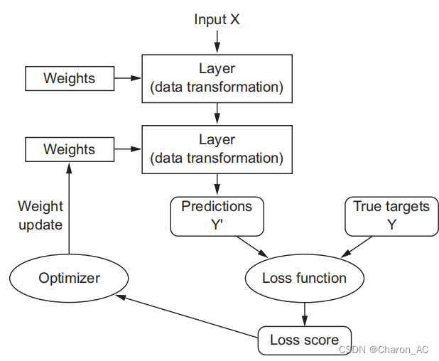
Layers
: the building blocks of deep learning
标红的为这几种情况常用方法
十二、简单介绍Keras
Keras有以下几个特点
1.它允许相同的代码在CPU或GPU上无缝运行。
2.它有一个用户友好的API,可以轻松地快速地原型深度学习模型。
3.它内置了对卷积网络(用于计算机视觉)、递归网络(用于序列处理)以及两者的任何组合的支持。
4.它支持任意的网络体系结构:多输入或多输出模型、图层共享、模型共享等。这意味着Keras基本上适用于构建任何深度学习模型,从生成式对抗网络到神经图灵机。
典型的Keras工作流:
1.定义训练数据:输入张量和目标张量。 tensors and target tensors
2.定义一个将输入映射到目标的层(或模型)网络。
3.通过选择损失函数、优化器和一些监控指标来配置学习过程。
4通过调用模型的fit()方法迭代训练数据。
这里有一个使用顺序类定义的两层模型(注意,我们正在将输入数据的预期形状传递给第一层):
from keras import models
from keras import layers
model = models.Sequential()
model.add(layers.Dense(32, activation='relu', input_shape=(784,)))
model.add(layers.Dense(10, activation='softmax'))
这里是使用函数API定义的相同模型:
input_tensor = layers.Input(shape=(784,))
x = layers.Dense(32, activation='relu')(input_tensor)
output_tensor = layers.Dense(10, activation='softmax')(x)
model = models.Model(inputs=input_tensor, outputs=output_tensor)


 1045
1045

 被折叠的 条评论
为什么被折叠?
被折叠的 条评论
为什么被折叠?
 到【灌水乐园】发言


