基础TensorFlow搭建的神经网络实现鸢尾花分类

     这是个多层神经网络来实现对鸢尾花数据的训练，来达到精准分类的目的

import tensorflow as tf
import numpy as np
import pandas as pd
import matplotlib.pyplot as plt
# print(tf.__version__)
from sklearn.datasets import load_iris
from sklearn.model_selection import train_test_split

#=======================多层神经网络==================================
# 加载鸢尾花数据集
iris = load_iris()
x = iris.data  # 特征数据
y = iris.target  # 标签数据

# 划分训练集和测试集
x_train, x_test, y_train, y_test = train_test_split(x, y, test_size=0.2, random_state=42)

# 数据预处理：标准化
x_train = x_train - np.mean(x_train, axis=0)
x_test = x_test - np.mean(x_test, axis=0)

# 转换为 TensorFlow 张量
X_train = tf.cast(x_train, tf.float32)
Y_train = tf.one_hot(tf.constant(y_train, dtype=tf.int32), 3)
X_test = tf.cast(x_test, tf.float32)
Y_test = tf.one_hot(tf.constant(y_test, dtype=tf.int32), 3)

# 设置超参数
learn__rate = 0.5         #学习率
iter = 50                 #训练次数
step = 10                 #步长
np.random.seed(612)       #初始化权重矩阵，生成一个服从标准正态分布（均值为0，标准差为1）的随机数组成的矩阵

# 初始化模型参数
W1 = tf.Variable(np.random.randn(4,8), dtype=tf.float32)
B1 = tf.Variable(np.zeros([8]), dtype=tf.float32)
W2 = tf.Variable(np.random.randn(8, 16), dtype=tf.float32)
B2 = tf.Variable(np.zeros([16]), dtype=tf.float32)
W3 = tf.Variable(np.random.randn(16, 3), dtype=tf.float32)
B3 = tf.Variable(np.zeros([3]), dtype=tf.float32)

# 存储训练过程中的准确率和损失值
acc_train = []
acc_test = []
cce_train = []
cce_test = []

# 迭代训练
for i in range(0, iter + 1):
    with tf.GradientTape() as tape:
        # 前向传播计算训练集上的预测值和损失
        Hiden_train1 = tf.nn.relu(tf.matmul(X_train, W1) + B1)
        Hiden_train2 = tf.nn.tanh(tf.matmul(Hiden_train1, W2) + B2)
        PRED_train = tf.nn.softmax(tf.matmul(Hiden_train2, W3) + B3)
        Loss_train = tf.reduce_mean(tf.keras.losses.categorical_crossentropy(y_true=Y_train, y_pred=PRED_train))

        # 前向传播计算测试集上的预测值和损失
        Hiden_test1 = tf.nn.relu(tf.matmul(X_test, W1) + B1)
        Hiden_test2 = tf.nn.tanh(tf.matmul(Hiden_test1, W2) + B2)
        PRED_test = tf.nn.softmax(tf.matmul(Hiden_test2, W3) + B3)
        Loss_test = tf.reduce_mean(tf.keras.losses.categorical_crossentropy(y_true=Y_test, y_pred=PRED_test))

    # 计算训练集和测试集的准确率
    accuracy_train = tf.reduce_mean(tf.cast(tf.equal(tf.argmax(PRED_train.numpy(), axis=1), y_train), tf.float32))
    accuracy_test = tf.reduce_mean(tf.cast(tf.equal(tf.argmax(PRED_test.numpy(), axis=1), y_test), tf.float32))

    # 存储准确率和损失值
    acc_train.append(accuracy_train)
    acc_test.append(accuracy_test)
    cce_train.append(Loss_train)
    cce_test.append(Loss_test)

    # 计算梯度并更新参数
    grads = tape.gradient(Loss_train, [W1,B1,W2,B2,W3,B3])
    W1.assign_sub(learn__rate * grads[0])
    B1.assign_sub(learn__rate * grads[1])
    W2.assign_sub(learn__rate * grads[2])
    B2.assign_sub(learn__rate * grads[3])
    W3.assign_sub(learn__rate * grads[4])
    B3.assign_sub(learn__rate * grads[5])

    # 打印训练过程中的指标
    if i % step == 0:
        print(i, accuracy_train, Loss_train, accuracy_test, Loss_test)

# 绘制损失和准确率曲线
plt.figure(figsize=(10, 3))
plt.subplot(121)
plt.plot(cce_train, color="blue", label="train")
plt.plot(cce_test, color="red", label="test")
plt.ylabel("loss")
plt.legend()

plt.subplot(122)
plt.plot(acc_train, color="blue", label="train")
plt.plot(acc_test, color="red", label="test")
plt.ylabel("accuracy")
plt.legend()

plt.show()

输出结果
0 tf.Tensor(0.4, shape=(), dtype=float32) tf.Tensor(2.0974417, shape=(), dtype=float32) tf.Tensor(0.56666666, shape=(), dtype=float32) tf.Tensor(1.5950611, shape=(), dtype=float32)
10 tf.Tensor(0.90833336, shape=(), dtype=float32) tf.Tensor(0.20110139, shape=(), dtype=float32) tf.Tensor(0.93333334, shape=(), dtype=float32) tf.Tensor(0.15459448, shape=(), dtype=float32)
20 tf.Tensor(0.94166666, shape=(), dtype=float32) tf.Tensor(0.15309285, shape=(), dtype=float32) tf.Tensor(0.96666664, shape=(), dtype=float32) tf.Tensor(0.10885302, shape=(), dtype=float32)
30 tf.Tensor(0.94166666, shape=(), dtype=float32) tf.Tensor(0.12801662, shape=(), dtype=float32) tf.Tensor(0.96666664, shape=(), dtype=float32) tf.Tensor(0.079918735, shape=(), dtype=float32)
40 tf.Tensor(0.9583333, shape=(), dtype=float32) tf.Tensor(0.10967161, shape=(), dtype=float32) tf.Tensor(1.0, shape=(), dtype=float32) tf.Tensor(0.060291704, shape=(), dtype=float32)
50 tf.Tensor(0.9583333, shape=(), dtype=float32) tf.Tensor(0.09543578, shape=(), dtype=float32) tf.Tensor(1.0, shape=(), dtype=float32) tf.Tensor(0.048254915, shape=(), dtype=float32)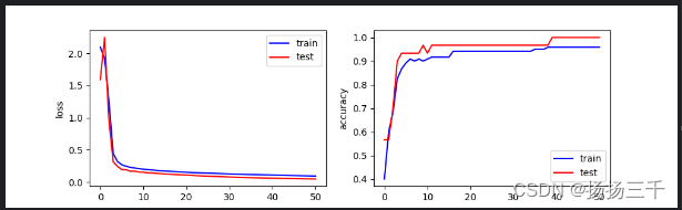

原理:

对特征数据进行标准化处理，即将每个特征的均值减去，以便加速模型的收敛。定义了一个包含3个隐藏层的多层神经网络，分别为输入层、两个隐藏层和输出层。使用 ReLU 和 tanh 激活函数来增加网络的非线性拟合能力。使用 TensorFlow 来定义模型的参数，并通过梯度下降算法来优化参数。计算训练集和测试集上的预测值和损失，并使用交叉熵作为损失函数。通过比较预测值和真实标签来计算准确率。

把数据分为训练集和测试集，前者占80%，后者占20%，

目的是看由训练集得到的参数是否过拟合。