


知识点回顾:
- 三种不同的模型可视化方法:推荐torchinfo打印summary+权重分布可视化
- 进度条功能:手动和自动写法,让打印结果更加美观
- 推理的写法:评估模式
import torch
import torch.nn as nn
import torch.optim as optim
from sklearn.datasets import load_iris
from sklearn.model_selection import train_test_split
from sklearn.preprocessing import MinMaxScaler
import time
import matplotlib.pyplot as plt

# 设置GPU设备
device = torch.device("cuda:0" if torch.cuda.is_available() else "cpu")
print(f"使用设备: {device}")

# 加载鸢尾花数据集
iris = load_iris()
X = iris.data  # 特征数据
y = iris.target  # 标签数据

# 划分训练集和测试集
X_train, X_test, y_train, y_test = train_test_split(X, y, test_size=0.2, random_state=42)

# 归一化数据
scaler = MinMaxScaler()
X_train = scaler.fit_transform(X_train)
X_test = scaler.transform(X_test)

# 将数据转换为PyTorch张量并移至GPU
X_train = torch.FloatTensor(X_train).to(device)
y_train = torch.LongTensor(y_train).to(device)
X_test = torch.FloatTensor(X_test).to(device)
y_test = torch.LongTensor(y_test).to(device)

class MLP(nn.Module):
    def __init__(self):
        super(MLP, self).__init__()
        self.fc1 = nn.Linear(4, 10)  # 输入层到隐藏层
        self.relu = nn.ReLU()
        self.fc2 = nn.Linear(10, 3)  # 隐藏层到输出层

    def forward(self, x):
        out = self.fc1(x)
        out = self.relu(out)
        out = self.fc2(out)
        return out

# 实例化模型并移至GPU
model = MLP().to(device)

# 分类问题使用交叉熵损失函数
criterion = nn.CrossEntropyLoss()

# 使用随机梯度下降优化器
optimizer = optim.SGD(model.parameters(), lr=0.01)

# 训练模型
num_epochs = 20000  # 训练的轮数

# 用于存储每100个epoch的损失值和对应的epoch数
losses = []

start_time = time.time()  # 记录开始时间

for epoch in range(num_epochs):
    # 前向传播
    outputs = model(X_train)  # 隐式调用forward函数
    loss = criterion(outputs, y_train)

    # 反向传播和优化
    optimizer.zero_grad() #梯度清零,因为PyTorch会累积梯度,所以每次迭代需要清零,梯度累计是那种小的bitchsize模拟大的bitchsize
    loss.backward() #  反向传播计算梯度
    optimizer.step() # 更新参数

    # 记录损失值
    if (epoch + 1) % 200 == 0:
        losses.append(loss.item()) # item()方法返回一个Python数值,loss是一个标量张量
        print(f'Epoch [{epoch+1}/{num_epochs}], Loss: {loss.item():.4f}')

    # 打印训练信息
    if (epoch + 1) % 100 == 0: # range是从0开始,所以epoch+1是从当前epoch开始,每100个epoch打印一次
        print(f'Epoch [{epoch+1}/{num_epochs}], Loss: {loss.item():.4f}')

time_all = time.time() - start_time  # 计算训练时间
print(f'Training time: {time_all:.2f} seconds')


# 可视化损失曲线
plt.plot(range(len(losses)), losses)
plt.xlabel('Epoch')
plt.ylabel('Loss')
plt.title('Training Loss over Epochs')
plt.show()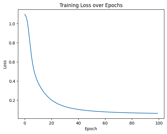
#  nn.Module 的内置功能,直接输出模型结构
print(model)


MLP(
  (fc1): Linear(in_features=4, out_features=10, bias=True)
  (relu): ReLU()
  (fc2): Linear(in_features=10, out_features=3, bias=True)
)


# nn.Module 的内置功能,返回模型的可训练参数迭代器
for name, param in model.named_parameters():
    print(f"Parameter name: {name}, Shape: {param.shape}")


Parameter name: fc1.weight, Shape: torch.Size([10, 4])
Parameter name: fc1.bias, Shape: torch.Size([10])
Parameter name: fc2.weight, Shape: torch.Size([3, 10])
Parameter name: fc2.bias, Shape: torch.Size([3])
# 提取权重数据
import numpy as np
weight_data = {}
for name, param in model.named_parameters():
if 'weight' in name:
weight_data[name] = param.detach().cpu().numpy()
# 可视化权重分布
fig, axes = plt.subplots(1, len(weight_data), figsize=(15, 5))
fig.suptitle('Weight Distribution of Layers')
for i, (name, weights) in enumerate(weight_data.items()):
# 展平权重张量为一维数组
weights_flat = weights.flatten()
# 绘制直方图
axes[i].hist(weights_flat, bins=50, alpha=0.7)
axes[i].set_title(name)
axes[i].set_xlabel('Weight Value')
axes[i].set_ylabel('Frequency')
axes[i].grid(True, linestyle='--', alpha=0.7)
plt.tight_layout()
plt.subplots_adjust(top=0.85)
plt.show()
# 计算并打印每层权重的统计信息
print("\n=== 权重统计信息 ===")
for name, weights in weight_data.items():
mean = np.mean(weights)
std = np.std(weights)
min_val = np.min(weights)
max_val = np.max(weights)
print(f"{name}:")
print(f" 均值: {mean:.6f}")
print(f" 标准差: {std:.6f}")
print(f" 最小值: {min_val:.6f}")
print(f" 最大值: {max_val:.6f}")
print("-" * 30)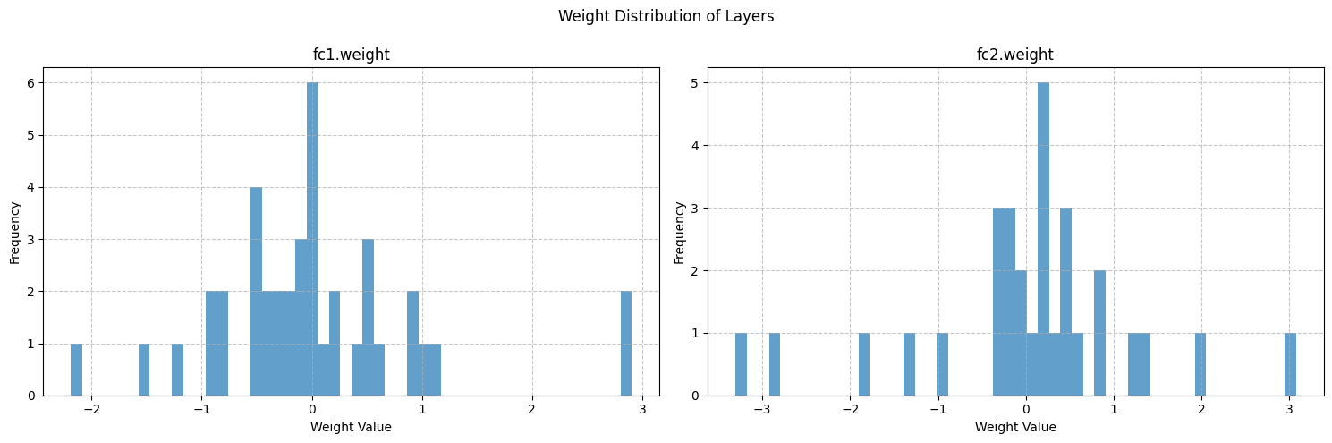
from torchsummary import summary
# 打印模型摘要,可以放置在模型定义后面
summary(model, input_size=(4,))


----------------------------------------------------------------
        Layer (type)               Output Shape         Param #
================================================================
            Linear-1                   [-1, 10]              50
              ReLU-2                   [-1, 10]               0
            Linear-3                    [-1, 3]              33
================================================================
Total params: 83
Trainable params: 83
Non-trainable params: 0
----------------------------------------------------------------
Input size (MB): 0.00
Forward/backward pass size (MB): 0.00
Params size (MB): 0.00
Estimated Total Size (MB): 0.00
----------------------------------------------------------------


from torchinfo import summary
summary(model, input_size=(4, ))


==========================================================================================
Layer (type:depth-idx)                   Output Shape              Param #
==========================================================================================
MLP                                      [3]                       --
├─Linear: 1-1                            [10]                      50
├─ReLU: 1-2                              [10]                      --
├─Linear: 1-3                            [3]                       33
==========================================================================================
Total params: 83
Trainable params: 83
Non-trainable params: 0
Total mult-adds (M): 0.00
==========================================================================================
Input size (MB): 0.00
Forward/backward pass size (MB): 0.00
Params size (MB): 0.00
Estimated Total Size (MB): 0.00
==========================================================================================
from tqdm import tqdm # 先导入tqdm库
import time # 用于模拟耗时操作
# 创建一个总步数为10的进度条
with tqdm(total=10) as pbar: # pbar是进度条对象的变量名
# pbar 是 progress bar(进度条)的缩写,约定俗成的命名习惯。
for i in range(10): # 循环10次(对应进度条的10步)
time.sleep(0.5) # 模拟每次循环耗时0.5秒
pbar.update(1) # 每次循环后,进度条前进1步
from tqdm import tqdm
import time
# 创建进度条时添加描述(desc)和单位(unit)
with tqdm(total=5, desc="下载文件", unit="个") as pbar:
# 进度条这个对象,可以设置描述和单位
# desc是描述,在左侧显示
# unit是单位,在进度条右侧显示
for i in range(5):
time.sleep(1)
pbar.update(1) # 每次循环进度+1
from tqdm import tqdm
import time
# 直接将range(3)传给tqdm,自动生成进度条
# 这个写法我觉得是有点神奇的,直接可以给这个对象内部传入一个可迭代对象,然后自动生成进度条
for i in tqdm(range(3), desc="处理任务", unit="epoch"):
time.sleep(1)
# 用tqdm的set_postfix方法在进度条右侧显示实时数据(如当前循环的数值、计算结果等):
from tqdm import tqdm
import time
total = 0 # 初始化总和
with tqdm(total=10, desc="累加进度") as pbar:
for i in range(1, 11):
time.sleep(0.3)
total += i # 累加1+2+3+...+10
pbar.update(1) # 进度+1
pbar.set_postfix({"当前总和": total}) # 显示实时总和
import torch
import torch.nn as nn
import torch.optim as optim
from sklearn.datasets import load_iris
from sklearn.model_selection import train_test_split
from sklearn.preprocessing import MinMaxScaler
import time
import matplotlib.pyplot as plt
from tqdm import tqdm # 导入tqdm库用于进度条显示
# 设置GPU设备
device = torch.device("cuda:0" if torch.cuda.is_available() else "cpu")
print(f"使用设备: {device}")
# 加载鸢尾花数据集
iris = load_iris()
X = iris.data # 特征数据
y = iris.target # 标签数据
# 划分训练集和测试集
X_train, X_test, y_train, y_test = train_test_split(X, y, test_size=0.2, random_state=42)
# 归一化数据
scaler = MinMaxScaler()
X_train = scaler.fit_transform(X_train)
X_test = scaler.transform(X_test)
# 将数据转换为PyTorch张量并移至GPU
X_train = torch.FloatTensor(X_train).to(device)
y_train = torch.LongTensor(y_train).to(device)
X_test = torch.FloatTensor(X_test).to(device)
y_test = torch.LongTensor(y_test).to(device)
class MLP(nn.Module):
def __init__(self):
super(MLP, self).__init__()
self.fc1 = nn.Linear(4, 10) # 输入层到隐藏层
self.relu = nn.ReLU()
self.fc2 = nn.Linear(10, 3) # 隐藏层到输出层
def forward(self, x):
out = self.fc1(x)
out = self.relu(out)
out = self.fc2(out)
return out
# 实例化模型并移至GPU
model = MLP().to(device)
# 分类问题使用交叉熵损失函数
criterion = nn.CrossEntropyLoss()
# 使用随机梯度下降优化器
optimizer = optim.SGD(model.parameters(), lr=0.01)
# 训练模型
num_epochs = 20000 # 训练的轮数
# 用于存储每100个epoch的损失值和对应的epoch数
losses = []
epochs = []
start_time = time.time() # 记录开始时间
# 创建tqdm进度条
with tqdm(total=num_epochs, desc="训练进度", unit="epoch") as pbar:
# 训练模型
for epoch in range(num_epochs):
# 前向传播
outputs = model(X_train) # 隐式调用forward函数
loss = criterion(outputs, y_train)
# 反向传播和优化
optimizer.zero_grad()
loss.backward()
optimizer.step()
# 记录损失值并更新进度条
if (epoch + 1) % 200 == 0:
losses.append(loss.item())
epochs.append(epoch + 1)
# 更新进度条的描述信息
pbar.set_postfix({'Loss': f'{loss.item():.4f}'})
# 每1000个epoch更新一次进度条
if (epoch + 1) % 1000 == 0:
pbar.update(1000) # 更新进度条
# 确保进度条达到100%
if pbar.n < num_epochs:
pbar.update(num_epochs - pbar.n) # 计算剩余的进度并更新
time_all = time.time() - start_time # 计算训练时间
print(f'Training time: {time_all:.2f} seconds')
# # 可视化损失曲线
# plt.figure(figsize=(10, 6))
# plt.plot(epochs, losses)
# plt.xlabel('Epoch')
# plt.ylabel('Loss')
# plt.title('Training Loss over Epochs')
# plt.grid(True)
# plt.show()# 在测试集上评估模型,此时model内部已经是训练好的参数了
# 评估模型
model.eval() # 设置模型为评估模式
with torch.no_grad(): # torch.no_grad()的作用是禁用梯度计算,可以提高模型推理速度
outputs = model(X_test) # 对测试数据进行前向传播,获得预测结果
_, predicted = torch.max(outputs, 1) # torch.max(outputs, 1)返回每行的最大值和对应的索引
#这个函数返回2个值,分别是最大值和对应索引,参数1是在第1维度(行)上找最大值,_ 是Python的约定,表示忽略这个返回值,所以这个写法是找到每一行最大值的下标
# 此时outputs是一个tensor,p每一行是一个样本,每一行有3个值,分别是属于3个类别的概率,取最大值的下标就是预测的类别
# predicted == y_test判断预测值和真实值是否相等,返回一个tensor,1表示相等,0表示不等,然后求和,再除以y_test.size(0)得到准确率
# 因为这个时候数据是tensor,所以需要用item()方法将tensor转化为Python的标量
# 之所以不用sklearn的accuracy_score函数,是因为这个函数是在CPU上运行的,需要将数据转移到CPU上,这样会慢一些
# size(0)获取第0维的长度,即样本数量
correct = (predicted == y_test).sum().item() # 计算预测正确的样本数
accuracy = correct / y_test.size(0)
print(f'测试集准确率: {accuracy * 100:.2f}%')


 5055
5055

 被折叠的 条评论
为什么被折叠?
被折叠的 条评论
为什么被折叠?
 到【灌水乐园】发言


