【无标题】python数学建模算法与应用课后习题

# 程序文件 ti5_7.py  
  
import cvxpy as cp  
import numpy as np  
import matplotlib.pyplot as plt  # 修正导入库  
  
# 定义优化变量  
x = cp.Variable(3, pos=True)  
  
# 定义约束条件  
constraints = [x[0] >= 0, sum(x[:2]) >= 100, sum(x) == 180]  
  
# 定义第一个优化问题  
obj0 = cp.Minimize(0.2 * sum(x ** 2) + 50 * sum(x) + 4 * (2 * x[0] + x[1] - 140))  
prob0 = cp.Problem(obj0, constraints)  
prob0.solve()  
print('最优值为：', prob0.value)  
print('最优解为：\n', x.value)  
  
# 初始化绘图数据  
plt.subplots_adjust(wspace=0.5)  
V1 = []  
for a in np.arange(40, 61, 2):  
    # 定义第二个优化问题（改变线性项的系数）  
    obj1 = cp.Minimize(0.2 * sum(x ** 2) + a * sum(x) + 4 * (2 * x[0] + x[1] - 140))  
    prob1 = cp.Problem(obj1, constraints)  
    prob1.solve()  
    V1.append(prob1.value)  
  
# 绘制第一个图  
plt.subplot(131)  
plt.plot(np.arange(40, 61, 2), V1)  
plt.title('Varying linear coefficient a')  
  
V2 = []  
for b in np.arange(0.15, 0.26, 0.01):  
    # 定义第三个优化问题（改变二次项的系数）  
    obj2 = cp.Minimize(b * sum(x ** 2) + 50 * sum(x) + 4 * (2 * x[0] + x[1] - 140))  
    prob2 = cp.Problem(obj2, constraints)  
    prob2.solve()  
    V2.append(prob2.value)  
  
# 绘制第二个图  
plt.subplot(132)  
plt.plot(np.arange(0.15, 0.26, 0.01), V2)  
plt.title('Varying quadratic coefficient b')  
  
V3 = []  
for c in np.arange(3, 5.1, 0.1):  
    # 定义第四个优化问题（改变某个特定线性组合的系数）  
    obj3 = cp.Minimize(0.2 * sum(x ** 2) + 50 * sum(x) + c * (2 * x[0] + x[1] - 140))  
    prob3 = cp.Problem(obj3, constraints)  
    prob3.solve()  
    V3.append(prob3.value)  
  
# 绘制第三个图  
plt.subplot(133)  
plt.plot(np.arange(3, 5.1, 0.1), V3)  
plt.title('Varying specific linear combination coefficient c')  
  
# 显示图形  
plt.show()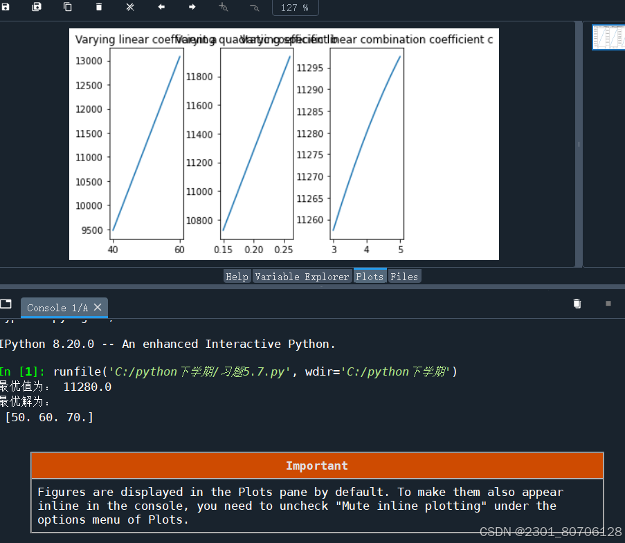

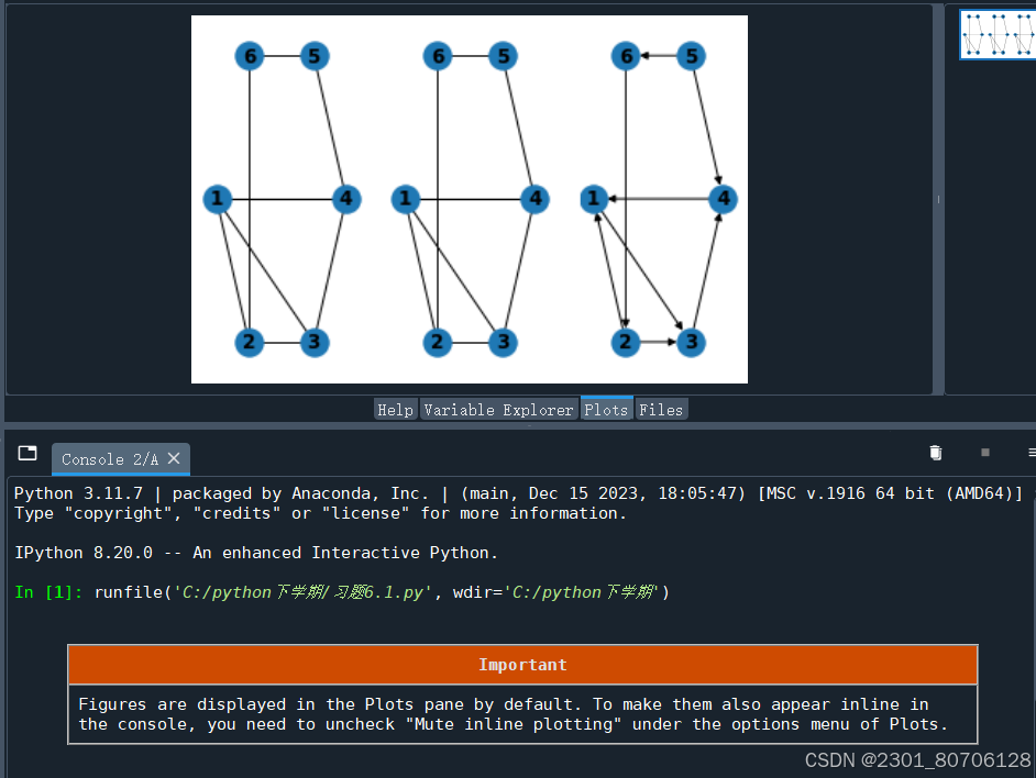
# 程序文件 ti6_1.py  

import networkx as nx 
import pylab as plt 

L1=[(1,2),(1,3),(1,4),(2,3),(2,6),(3,4),(4,5),(5,6)]
G1= nx.Graph ();G1.add_nodes_from ( range (1,7))
G1.add_edges_from(L1);pos1=nx.shell_layout(G1)
plt.subplot (131)
nx.draw(G1,pos1,with_labels=True,font_weight='bold')

L2=[(1,2,7),(1,3,3),(1,4,12),(2,3,1),(2,6,1),(3,4,8),(4,5,9),(5,6,3)]
G2= nx.Graph();G2.add_nodes_from(range(1,7))
G2.add_weighted_edges_from(L2);pos2=nx.shell_layout(G2)
plt.subplot(132)
nx.draw(G2,pos2,with_labels=True,font_weight='bold')
w2=nx.get_edge_attributes(G2,'weight ')
nx.draw_networkx_edge_labels(G2,pos2,edge_labels =w2)

L3=[(1,3,3),(2,1,7),(2,3,1),(3,4,8),(4,1,12),(5,4,9),(5,6,3),(6,2,1)]
G3=nx.DiGraph();G3.add_nodes_from(range(1,7))
G3.add_weighted_edges_from(L3);pos3=nx.shell_layout(G3)
plt.subplot(133)
nx.draw(G3,pos3,with_labels=True,font_weight='bold')
w3= nx.get_edge_attributes(G3,' weight ')
nx.draw_networkx_edge_labels(G3,pos3,edge_labels =w3)
plt.show ()

# 程序文件 ti6_3.py  
import numpy as np  
import networkx as nx  
import matplotlib.pyplot as plt  # 导入绘图库  
  
L = [(1, 2, 20), (1, 5, 15), (2, 3, 20), (2, 4, 60), (2, 5, 25),  
     (3, 4, 30), (3, 5, 18), (4, 5, 35), (4, 6, 10), (5, 6, 15)]  
G = nx.Graph()  
G.add_nodes_from(range(1, 7))  
G.add_weighted_edges_from(L)  
  
T = nx.minimum_spanning_tree(G)  
w = nx.get_edge_attributes(T, 'weight')  
TL = sum(w.values())  
print('最小生成树的长度:', TL)  
  
pos = nx.shell_layout(G)  
s = ['v' + str(i) for i in range(1, 7)]  
s = dict(zip(range(1, 7), s))  # 这一步其实是多余的，因为可以直接在draw中使用labels参数  
  
# 绘制最小生成树  
nx.draw(T, pos, labels=s, with_labels=True, node_color='lightblue', node_size=500, font_weight='bold')  
nx.draw_networkx_edge_labels(T, pos, edge_labels=w)  
  
plt.show()

# 程序文件 ti6_4.py  

import numpy as np 
import networkx as nx 
import pylab as plt 
a = np . zeros ((5,5))

a[0,1:]=[0.8,2,3.8,6]
a[1,2:]=[0.9,2.1,3.9]
a[2,3:]=[1.1,2.3]; a [3,4]=1.4
G=nx.DiGraph ( a )
p=nx.shortest_path(G,0,4, weight =' weight ')

d =nx.shortest_path_length( G ,0,4, weight =' weight ')
print ('最短路径为：', np . array ( p )+1)
print ('最小费用为：', d )

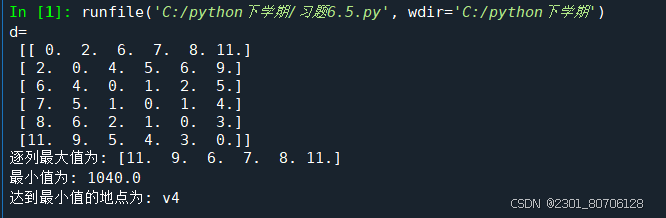
# 程序文件 ti6_5.py  
import numpy as np  
import networkx as nx  
import pandas as pd  
import matplotlib.pyplot as plt  
n = 6  
node = ['v' + str(i) for i in range(1, n + 1)]  
A = np.zeros((n, n))  
A[0, [1, 2]] = [2, 7]  
A[1, 2:5] = [4, 6, 8]  
A[2, [3, 4]] = [1, 3]  
A[3, [4, 5]] = [1, 6]  
A[4, 5] = 3  
    
G = nx.Graph(A)  
    
d = nx.floyd_warshall_numpy(G)  
dm1 = np.max(d, axis=0)  
print('d= \n', d)  
print('逐列最大值为:', dm1)  
  
f = pd.ExcelWriter('ti6_5.xlsx')  
dd = pd.DataFrame(d)  
dd.to_excel(f, 'Sheet1', index=False)  
  
num = np.array([[50, 40, 60, 20, 70, 90]]).T   
D = num * d    
DD = pd.DataFrame(D)  
DD.to_excel(f, 'Sheet2', index=False)  
  
sd = np.sum(D, axis=0)  
sdm = np.min(sd)   
ind = np.argmin(sd)   
f.close()  
print('最小值为:', sdm)  
print('达到最小值的地点为:', node[ind])